metan 1.13.0 available now!
 Image by Larisa Koshkina on Pixabay
After exactly two months since the last stable release, I’m so proud to announce that metan 1.13.0 is now on
CRAN. This version includes important new features and bug corrections. In the last months, I’ve been receiving a lot of positive feedbacks and very useful suggestions to improve the package. Thanks to all!
metan was first released on CRAN on 2020/01/14 and since there, 12 stable versions have been released regularly. I’m happy with the results and the package now provides the main tools for manipulating, summarizing, analyzing, and plotting multi-environment trial data in plant breeding.
I need to inform you that due to my dedication to teaching and other new projects, I do not intend to plan a new stable release at least for the next few months. Critical bugs and the inclusion of new minor features will be added in the development version.
Instalation
# The latest stable version is installed with
install.packages("metan")

# Or the development version from GitHub:
# install.packages("devtools")
devtools::install_github("TiagoOlivoto/metan")
New functions
Utilities
progress()andrun_progress()for text progress bar in the terminal. A simple progress bar was included and the dependence of progress package removed.
library(metan)
# Registered S3 method overwritten by 'GGally':
#   method from
#   +.gg   ggplot2
# |========================================================|
# | Multi-Environment Trial Analysis (metan) v1.13.0       |
# | Author: Tiago Olivoto                                  |
# | Type 'citation('metan')' to know how to cite metan     |
# | Type 'vignette('metan_start')' for a short tutorial    |
# | Visit 'https://bit.ly/2TIq6JE' for a complete tutorial |
# |========================================================|
# Initialize the progress bar out of a loop
pb <-  progress(max = 10)
for (i in 1:10) {
# call the progress bar inside a loop
 run_progress(pb, actual = i)
}
#  |=======                                                                 | 10%
 |==============                                                          | 20%
 |======================                                                  | 30%
 |=============================                                           | 40%
 |====================================                                    | 50%
 |===========================================                             | 60%
 |==================================================                      | 70%
 |==========================================================              | 80%
 |=================================================================       | 90%
 |========================================================================| 100%

# More examples
# Shows a progress bar without percentage or elapsed time.
pb <-  progress(max = 5, style = 1)
for (i in 1:5) {
 run_progress(pb, actual = i,
              text = paste("Processing item", i))
}
# Processing item 1 |============                                                 |
Processing item 2 |========================                                     |
Processing item 3 |=====================================                        |
Processing item 4 |=================================================            |
Processing item 5 |=============================================================|

# Shows the progress bar and elapsed time.
pb <-  progress(max = 5, style = 3)
for (i in 1:5) {
 run_progress(pb, actual = i,
              sleep = 1,
              text = paste("Processing item", i))
}
# Processing item 1 |==========                                          | 00:00:01
Processing item 2 |=====================                               | 00:00:02
Processing item 3 |===============================                     | 00:00:03
Processing item 4 |==========================================          | 00:00:04
Processing item 5 |====================================================| 00:00:05

# Shows the progress bar, percentage, and elapsed time.
pb <-  progress(max = 5,
                style = 4,
                char = ".",
                rightd = "")
for (i in 1:5) {
 run_progress(pb, actual = i,
              sleep = 1,
              text = paste("Processing item", i))
}
# Processing item 1 |.........                                       20% 00:00:01
Processing item 2 |...................                             40% 00:00:02
Processing item 3 |............................                    60% 00:00:03
Processing item 4 |......................................          80% 00:00:04
Processing item 5 |............................................... 100% 00:00:05
rbind_fill_id()To implement the common pattern ofdo.call(rbind, dfs)with data
(df1 <- data.frame(v1 = c(1, 2), v2 = c(2, 3)))
#   v1 v2
# 1  1  2
# 2  2  3
(df2 <- data.frame(v3 = c(4, 5)))
#   v3
# 1  4
# 2  5
rbind_fill_id(df1, df2,
             .id = "dfs")
#   dfs v1 v2 v3
# 1 df1  1  2 NA
# 2 df1  2  3 NA
# 3 df2 NA NA  4
# 4 df2 NA NA  5
BLUP-based indexes
hmgv(),rpgv(),hmrpgv(),blup_indexes()to compute stability indexes based on a mixed-effect model.
In this version, Resende_indexes() was deprecated in favour of blup_indexes()
res_ind <- waasb(data_ge,
                 env = ENV,
                 gen = GEN,
                 rep = REP,
                 resp = c(GY, HM),
                 verbose = FALSE)
model_indexes <- blup_indexes(res_ind)
rbind_fill_id(model_indexes, .id = "TRAITS") %>% round_cols()
# # A tibble: 20 x 13
#    TRAITS GEN       Y  HMGV HMGV_R  RPGV RPGV_Y RPGV_R HMRPGV HMRPGV_Y HMRPGV_R
#    <chr>  <chr> <dbl> <dbl>  <dbl> <dbl>  <dbl>  <dbl>  <dbl>    <dbl>    <dbl>
#  1 GY     G1     2.6   2.32      6  0.97   2.59      6   0.97     2.59        6
#  2 GY     G10    2.47  2.11     10  0.91   2.44     10   0.9      2.4        10
#  3 GY     G2     2.74  2.47      4  1.03   2.74      4   1.02     2.73        4
#  4 GY     G3     2.96  2.68      2  1.11   2.96      2   1.1      2.95        2
#  5 GY     G4     2.64  2.39      5  0.99   2.65      5   0.99     2.64        5
#  6 GY     G5     2.54  2.3       8  0.95   2.55      7   0.95     2.55        8
#  7 GY     G6     2.53  2.3       7  0.95   2.55      8   0.95     2.55        7
#  8 GY     G7     2.74  2.52      3  1.04   2.77      3   1.03     2.76        3
#  9 GY     G8     3     2.74      1  1.13   3.01      1   1.12     3           1
# 10 GY     G9     2.51  2.18      9  0.93   2.48      9   0.92     2.45        9
# 11 HM     G1    47.1  46.9       9  0.98  47.2       9   0.98    47.2         9
# 12 HM     G10   48.5  48.0       4  1.01  48.4       4   1.01    48.4         4
# 13 HM     G2    46.7  46.5      10  0.97  46.8      10   0.97    46.8        10
# 14 HM     G3    47.6  47.3       8  0.99  47.6       8   0.99    47.6         8
# 15 HM     G4    48.0  47.8       5  1     48.1       5   1       48.0         5
# 16 HM     G5    49.3  48.9       1  1.02  49.2       1   1.02    49.2         1
# 17 HM     G6    48.7  48.4       3  1.01  48.7       3   1.01    48.6         3
# 18 HM     G7    48.0  47.7       6  1     48         6   1       48.0         6
# 19 HM     G8    49.1  48.7       2  1.02  49.0       2   1.02    49           2
# 20 HM     G9    47.9  47.5       7  1     47.9       7   1       47.8         7
# # ... with 2 more variables: WAASB <dbl>, WAASB_R <dbl>
Mean performance and stability
mps()andmtmps()for uni- and multivariate-based mean performance and stability
In one of my proposals to analyze stability and performance together, the WAASBY index has a critical limitation. Since WAASB is based on a singular value decomposition of the BLUPs for GE interaction, the two-way matrix must be complete, i.e., the trial must be balanced (all genotypes present in all environments). In the case of unbalanced data, imputation of missing values is needed to compute the WAASB index. If only a few cells need to be imputed, we have no major problems. Sometimes, however, highly unbalanced data is observed, and imputation may provide biased results. In this release, I have extended the theoretical foundations of the WAASBY index so that mean performance and stability could be computed with any stability index available in metan, including stability indexes that by theory don’t require a balanced trial.
Minor improvements
Bug fixes
-
blup_indexes()now removeNAs before computing harmonic and arithmetic means. -
Fix bug in
clustering()when using withbyargument and defacultnclustargument.
Minor improvements
-
mgidi()now have an optionalweightsargument to assign different weights for each trait in the selection process. Thanks to @MichelSouza for his suggestion. -
Licecycle badges added to the functions’ documentation.
-
Improved outputs in
plot_scoresthat now has ahighlightargument to highlight genotypes or environments by hand. Thanks to Ibrahim Elbasyoni for his suggestions.
As a motivating example, I’ll simulate a data with 120 genotypes and 6 environments, with 3 traits using ge_simula(). Then, compute the mixed-effect model with waasb() and the MTSI index with mtsi().
library(metan)
df <- ge_simula(ngen = 120,
                nenv = 6,
                nrep = 3,
                nvars = 3,
                seed = 1:3) # ensure reproducibility
# Warning: 'gen_eff = 20' recycled for all the 3 traits.
# Warning: 'env_eff = 15' recycled for all the 3 traits.
# Warning: 'rep_eff = 5' recycled for all the 3 traits.
# Warning: 'ge_eff = 10' recycled for all the 3 traits.
# Warning: 'res_eff = 5' recycled for all the 3 traits.
# Warning: 'intercept = 100' recycled for all the 3 traits.
mtsi_model <- waasb(df,
                    env = ENV,
                    gen = GEN,
                    rep = REP,
                    resp = everything())
# Evaluating trait V1 |===============                             | 33% 00:00:00
Evaluating trait V2 |=============================               | 67% 00:00:01
Evaluating trait V3 |============================================| 100% 00:00:01
# Method: REML/BLUP
# Random effects: GEN, GEN:ENV
# Fixed effects: ENV, REP(ENV)
# Denominador DF: Satterthwaite's method
# ---------------------------------------------------------------------------
# P-values for Likelihood Ratio Test of the analyzed traits
# ---------------------------------------------------------------------------
#     model        V1        V2        V3
#  COMPLETE        NA        NA        NA
#       GEN 2.86e-136 4.54e-153 9.35e-146
#   GEN:ENV 3.16e-125 1.52e-142 2.95e-146
# ---------------------------------------------------------------------------
# All variables with significant (p < 0.05) genotype-vs-environment interaction
mtsi_index <- mtsi(mtsi_model)
#
# -------------------------------------------------------------------------------
# Principal Component Analysis
# -------------------------------------------------------------------------------
# # A tibble: 3 x 4
#   PC    Eigenvalues `Variance (%)` `Cum. variance (%)`
#   <chr>       <dbl>          <dbl>               <dbl>
# 1 PC1         1.25            41.5                41.5
# 2 PC2         1.04            34.7                76.3
# 3 PC3         0.712           23.7               100
# -------------------------------------------------------------------------------
# Factor Analysis - factorial loadings after rotation-
# -------------------------------------------------------------------------------
# # A tibble: 3 x 5
#   VAR       FA1    FA2 Communality Uniquenesses
#   <chr>   <dbl>  <dbl>       <dbl>        <dbl>
# 1 V1    0.00404  0.952       0.906       0.0944
# 2 V2    0.799   -0.249       0.701       0.299
# 3 V3    0.778    0.277       0.682       0.318
# -------------------------------------------------------------------------------
# Comunalit Mean: 0.7627497
# -------------------------------------------------------------------------------
# Selection differential for the  waasby index
# -------------------------------------------------------------------------------
# # A tibble: 3 x 6
#   VAR   Factor    Xo    Xs    SD SDperc
#   <chr> <chr>  <dbl> <dbl> <dbl>  <dbl>
# 1 V2    FA 1    54.1  64.6  10.5   19.5
# 2 V3    FA 1    55.1  75.1  20.1   36.5
# 3 V1    FA 2    50.5  66.5  16.0   31.7
# -------------------------------------------------------------------------------
# Selection differential for the mean of the variables
# -------------------------------------------------------------------------------
# # A tibble: 3 x 11
#   VAR   Factor    Xo    Xs    SD SDperc    h2    SG SGperc sense     goal
#   <chr> <chr>  <dbl> <dbl> <dbl>  <dbl> <dbl> <dbl>  <dbl> <chr>    <dbl>
# 1 V2    FA 1   103.   108.  5.14   5.02 0.953  4.90   4.78 increase   100
# 2 V3    FA 1   101.   112. 11.1   11.0  0.950 10.5   10.5  increase   100
# 3 V1    FA 2    99.9  108.  7.70   7.71 0.945  7.27   7.28 increase   100
# ------------------------------------------------------------------------------
# Selected genotypes
# -------------------------------------------------------------------------------
# H88 H111 H55 H70 H73 H31 H94 H13 H9 H79 H74 H65 H10 H51 H40 H47 H7 H98
# -------------------------------------------------------------------------------
Note that plots with a relatively large number of lines are messy, and a warning “ggrepel: xx unlabeled data points (too many overlaps)" will occour.
plot_scores(mtsi_model, type = 3)
# Warning: ggrepel: 99 unlabeled data points (too many overlaps). Consider
# increasing max.overlaps
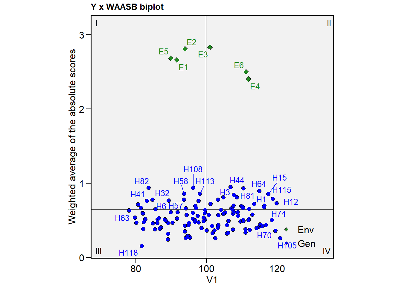
In this cases, I strongly suggest using repel = FALSE and reduce the size of the shapes and/or labels for environments/genotypes. We can do that now by using size.shape.* and size.tex.* arguments.
plot_scores(mtsi_model,
            type = 3,
            repel = FALSE,
            size.shape.gen = 1.5,
            size.tex.gen = 1.5)
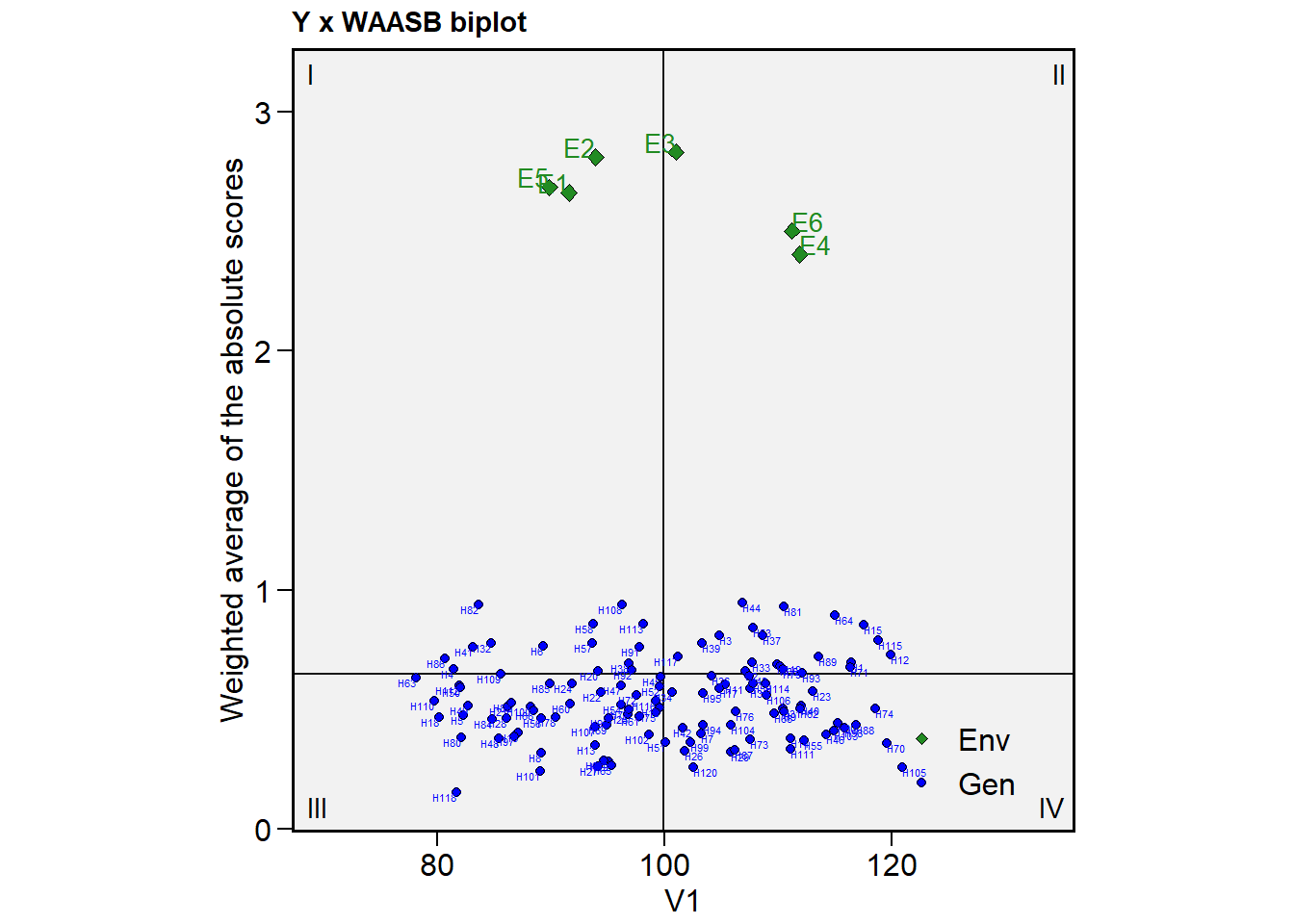
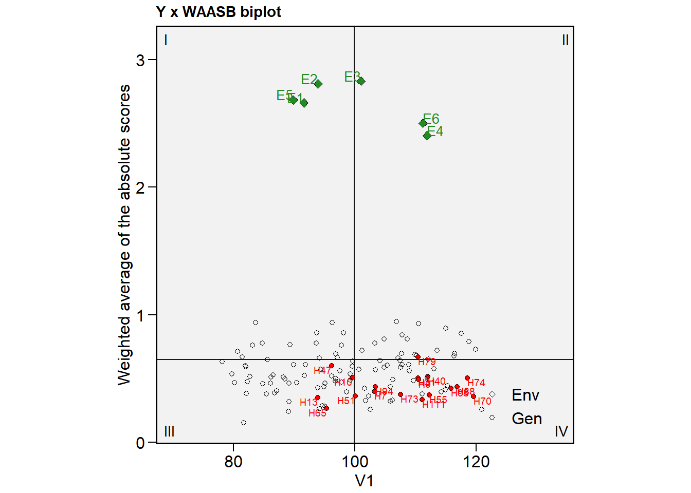
Still a bit messy, isn’t it? In the case when only some genotypes/environments are to be shown, we can use the highlight argument. Combining it with col.gen = transparent_color(), a little more tidy biplot can be produced. Note that highlight argument needs a vector of labels that must match the labels for genotypes/environments. Using sel_gen(), we can extract the selected genotypes by the MTSI index easily.
(selected <- sel_gen(mtsi_index))
#  [1] "H88"  "H111" "H55"  "H70"  "H73"  "H31"  "H94"  "H13"  "H9"   "H79"
# [11] "H74"  "H65"  "H10"  "H51"  "H40"  "H47"  "H7"   "H98"
plot_scores(mtsi_model,
            type = 3,
            repel = FALSE,
            size.shape.gen = 1.5,
            size.tex.gen = 2.5,
            col.gen = transparent_color(),
            highlight = selected,
            col.highlight = "red") # default
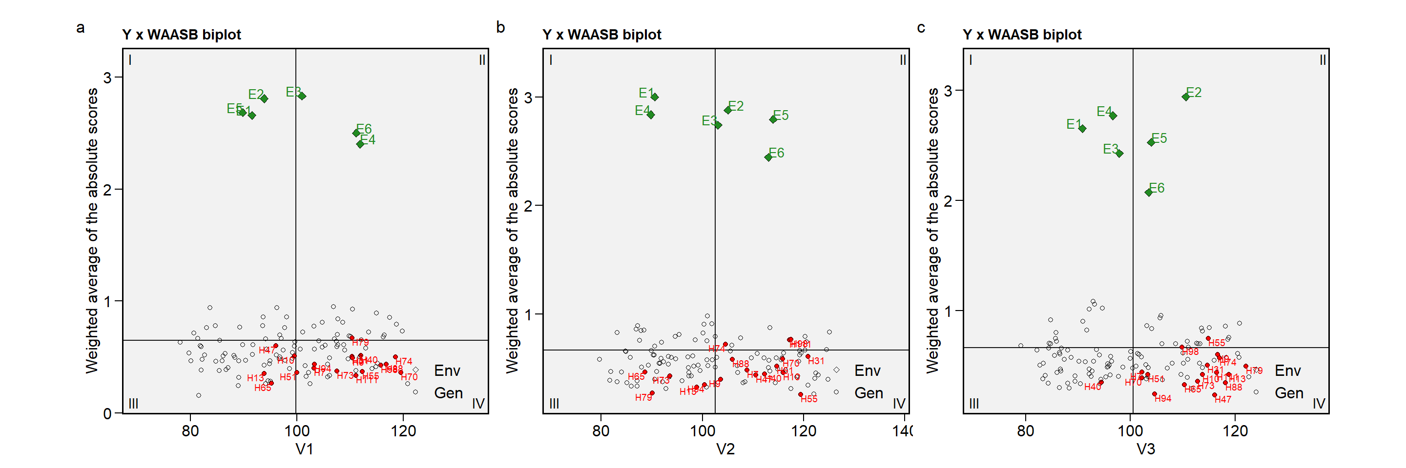
Showing the plot for all traits would look like something as follows
a <-
plot_scores(mtsi_model,
            type = 3,
            repel = FALSE,
            size.shape.gen = 1.5,
            size.tex.gen = 2.5,
            col.gen = transparent_color(),
            highlight = sel_gen(mtsi_index),
            col.highlight = "red") # default
b <-
plot_scores(mtsi_model,
            type = 3,
            var = 2,
            repel = FALSE,
            size.shape.gen = 1.5,
            size.tex.gen = 2.5,
            col.gen = transparent_color(),
            highlight = sel_gen(mtsi_index),
            col.highlight = "red") # default
c <-
plot_scores(mtsi_model,
            type = 3,
            var = 3,
            repel = FALSE,
            size.shape.gen = 1.5,
            size.tex.gen = 2.5,
            col.gen = transparent_color(),
            highlight = sel_gen(mtsi_index),
            col.highlight = "red") # default
arrange_ggplot(a, b, c,
               tag_levels = "a")
ge_reg()now returns hypotesis testing for slope and deviations from the regression. Thanks to @LeonardoBehring and @MichelSouza for the suggestion.
reg <- ge_reg(data_ge2,
             env = ENV,
             gen = GEN,
             rep = REP,
             resp = EH)
# Evaluating trait EH |============================================| 100% 00:00:00
print(reg)
# Variable EH
# ---------------------------------------------------------------------------
# Joint-regression Analysis of variance
# ---------------------------------------------------------------------------
# # A tibble: 20 x 6
#    SV                       Df `Sum Sq` `Mean Sq` `F value`    `Pr(>F)`
#    <chr>                 <dbl>    <dbl>     <dbl>     <dbl>       <dbl>
#  1 "Total"                  51  10.4       0.204     NA     NA
#  2 "GEN"                    12   1.03      0.0856     0.578  0.840
#  3 "ENV + (GEN x ENV)"      39   9.40      0.241     NA     NA
#  4 "ENV (linear)"            1   5.06      5.06      NA     NA
#  5 " GEN x ENV (linear)"    12   0.482     0.0402     0.271  0.989
#  6 "Pooled deviation"       26   3.85      0.148     NA     NA
#  7 "H1"                      2   0.424     0.212     10.2    0.0000949
#  8 "H10"                     2   0.223     0.112      5.38   0.00611
#  9 "H11"                     2   0.195     0.0976     4.71   0.0112
# 10 "H12"                     2   0.558     0.279     13.5    0.00000707
# 11 "H13"                     2   0.220     0.110      5.31   0.00652
# 12 "H2"                      2   0.630     0.315     15.2    0.00000186
# 13 "H3"                      2   0.564     0.282     13.6    0.00000637
# 14 "H4"                      2   0.242     0.121      5.84   0.00403
# 15 "H5"                      2   0.0684    0.0342     1.65   0.198
# 16 "H6"                      2   0.105     0.0526     2.54   0.0845
# 17 "H7"                      2   0.134     0.0672     3.24   0.0435
# 18 "H8"                      2   0.459     0.230     11.1    0.0000472
# 19 "H9"                      2   0.0287    0.0144     0.693  0.503
# 20 "Pooled error"           96   1.99      0.0207    NA     NA
# ---------------------------------------------------------------------------
# Regression parameters
# ---------------------------------------------------------------------------
# # A tibble: 13 x 10
#    GEN      b0    b1 `t(b1=1)`[,1] pval_t[,1]     s2di `F(s2di=0)`     pval_f
#    <chr> <dbl> <dbl>         <dbl>      <dbl>    <dbl>       <dbl>      <dbl>
#  1 H1     1.50 1.06        0.269       0.789   0.0637       10.2   0.0000949
#  2 H10    1.26 1.30        1.30        0.195   0.0303        5.38  0.00611
#  3 H11    1.27 1.00        0.00622     0.995   0.0256        4.71  0.0112
#  4 H12    1.28 0.590      -1.78        0.0785  0.0861       13.5   0.00000707
#  5 H13    1.35 0.575      -1.84        0.0687  0.0298        5.31  0.00652
#  6 H2     1.38 0.525      -2.06        0.0422  0.0981       15.2   0.00000186
#  7 H3     1.41 1.15        0.636       0.526   0.0870       13.6   0.00000637
#  8 H4     1.43 1.41        1.76        0.0820  0.0335        5.84  0.00403
#  9 H5     1.37 1.30        1.29        0.201   0.00449       1.65  0.198
# 10 H6     1.41 0.780      -0.952       0.343   0.0106        2.54  0.0845
# 11 H7     1.32 0.950      -0.219       0.827   0.0155        3.24  0.0435
# 12 H8     1.21 0.886      -0.495       0.621   0.0696       11.1   0.0000472
# 13 H9     1.27 1.48        2.08        0.0399 -0.00212       0.693 0.503
# # ... with 2 more variables: RMSE <dbl>, R2 <dbl>
# ---------------------------------------------------------------------------
# Variance of b0: 0.001728521
# Variance of b1: 0.05328109
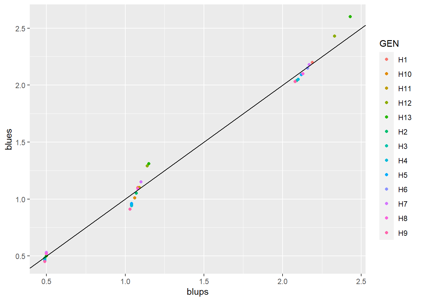
get_model_data()now extract BLUEs from objects computed withgamem()andgamem_met(). Thanks to @MdFarhad for suggesting me this improvement.
mix_mod <-
  gamem(data_g, GEN, REP, PH:EP, verbose = FALSE)
(blups <- gmd(mix_mod, "blupg") %>% round_cols())
# # A tibble: 13 x 4
#    GEN      PH    EH    EP
#    <chr> <dbl> <dbl> <dbl>
#  1 H1     2.19  1.08  0.5
#  2 H10    2.09  1.06  0.5
#  3 H11    2.13  1.09  0.5
#  4 H12    2.33  1.14  0.5
#  5 H13    2.43  1.15  0.5
#  6 H2     2.16  1.07  0.49
#  7 H3     2.09  1.04  0.49
#  8 H4     2.1   1.04  0.49
#  9 H5     2.12  1.04  0.49
# 10 H6     2.16  1.1   0.5
# 11 H7     2.17  1.1   0.5
# 12 H8     2.13  1.08  0.5
# 13 H9     2.08  1.03  0.49
(blues <- gmd(mix_mod, "blueg") %>% round_cols())
# # A tibble: 13 x 4
#    GEN      PH    EH    EP
#    <fct> <dbl> <dbl> <dbl>
#  1 H1     2.2   1.1   0.5
#  2 H10    2.04  1.01  0.5
#  3 H11    2.1   1.1   0.52
#  4 H12    2.43  1.29  0.52
#  5 H13    2.6   1.31  0.5
#  6 H2     2.15  1.05  0.48
#  7 H3     2.04  0.95  0.47
#  8 H4     2.05  0.94  0.46
#  9 H5     2.09  0.96  0.46
# 10 H6     2.15  1.15  0.53
# 11 H7     2.18  1.15  0.53
# 12 H8     2.1   1.09  0.52
# 13 H9     2.03  0.91  0.45

library(tidyverse)
df1 <- pivot_longer(blups, - GEN)
df2 <- pivot_longer(blues, - GEN)
bind <- left_join(df1, df2, by = c("GEN", "name"))
ggplot(bind, aes(value.x, value.y, color = GEN)) +
  geom_point() +
  geom_abline(intercept = 0, slope = 1) +
  labs(x = "blups", y = "blues")
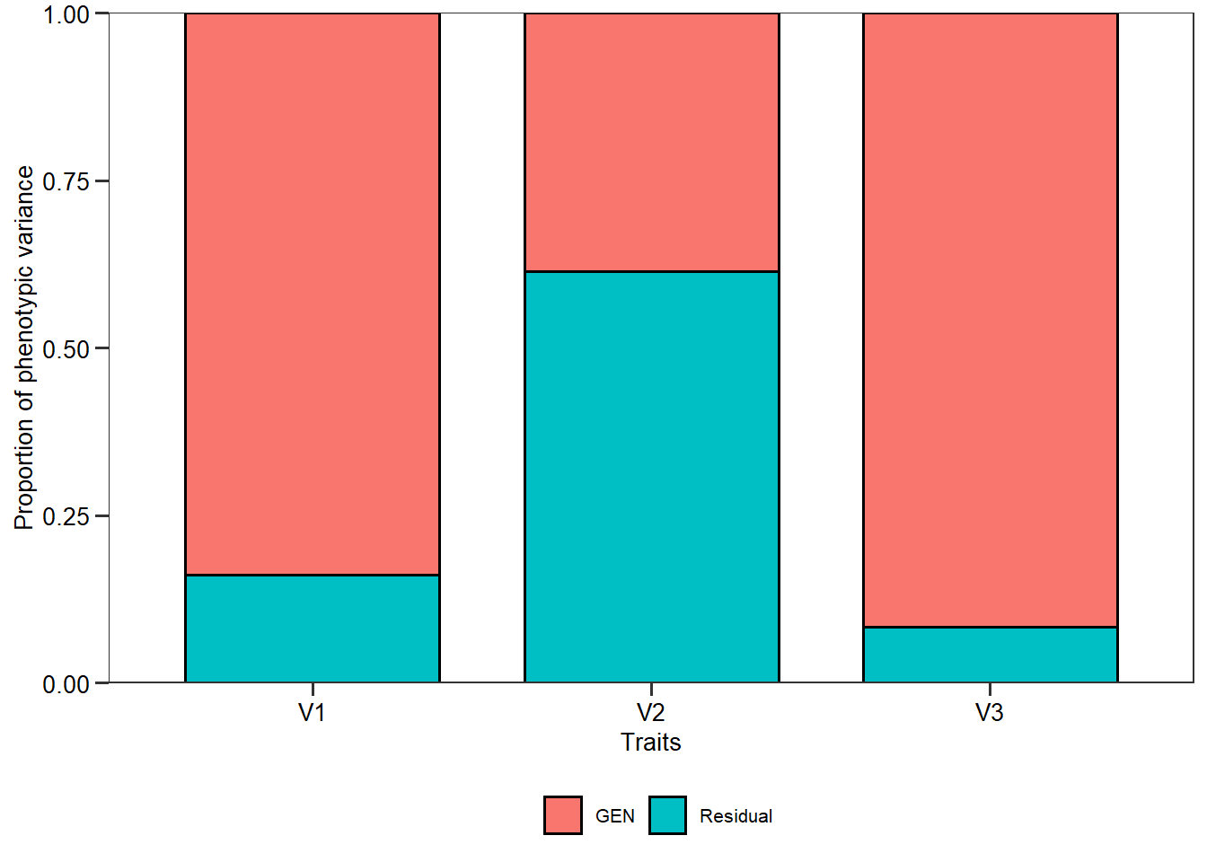
g_simula()andge_simula()now have ares_effto control the residual effect.
gen_data <-
   g_simula(ngen = 5,
            nrep = 3,
            nvars = 3,
            res_eff = c(4, 20, 4),
            seed = 1:3)
# Warning: 'gen_eff = 20' recycled for all the 3 traits.
# Warning: 'rep_eff = 5' recycled for all the 3 traits.
# Warning: 'intercept = 100' recycled for all the 3 traits.
gen_data
# # A tibble: 15 x 5
#    GEN   REP      V1    V2    V3
#    <fct> <fct> <dbl> <dbl> <dbl>
#  1 H1    B1     95.9  90.2  88.5
#  2 H1    B2     91.8  86.3  83.1
#  3 H1    B3     94.2 105.   85.0
#  4 H2    B1    102.  108.  118.
#  5 H2    B2    102.  144.  104.
#  6 H2    B3     95.3 109.  115.
#  7 H3    B1    113.  116.   93.5
#  8 H3    B2    109.  119.   87.1
#  9 H3    B3    102.   98.4  90.5
# 10 H4    B1    111.   70.4  95.2
# 11 H4    B2    125.  119.   90.0
# 12 H4    B3    118.   43.8  89.8
# 13 H5    B1     92.0 140.  101.
# 14 H5    B2     96.3 115.   97.7
# 15 H5    B3     93.0 141.  107.

mod <- gamem(gen_data, GEN, REP, everything(), verbose = FALSE)
plot(mod, type = "vcomp")
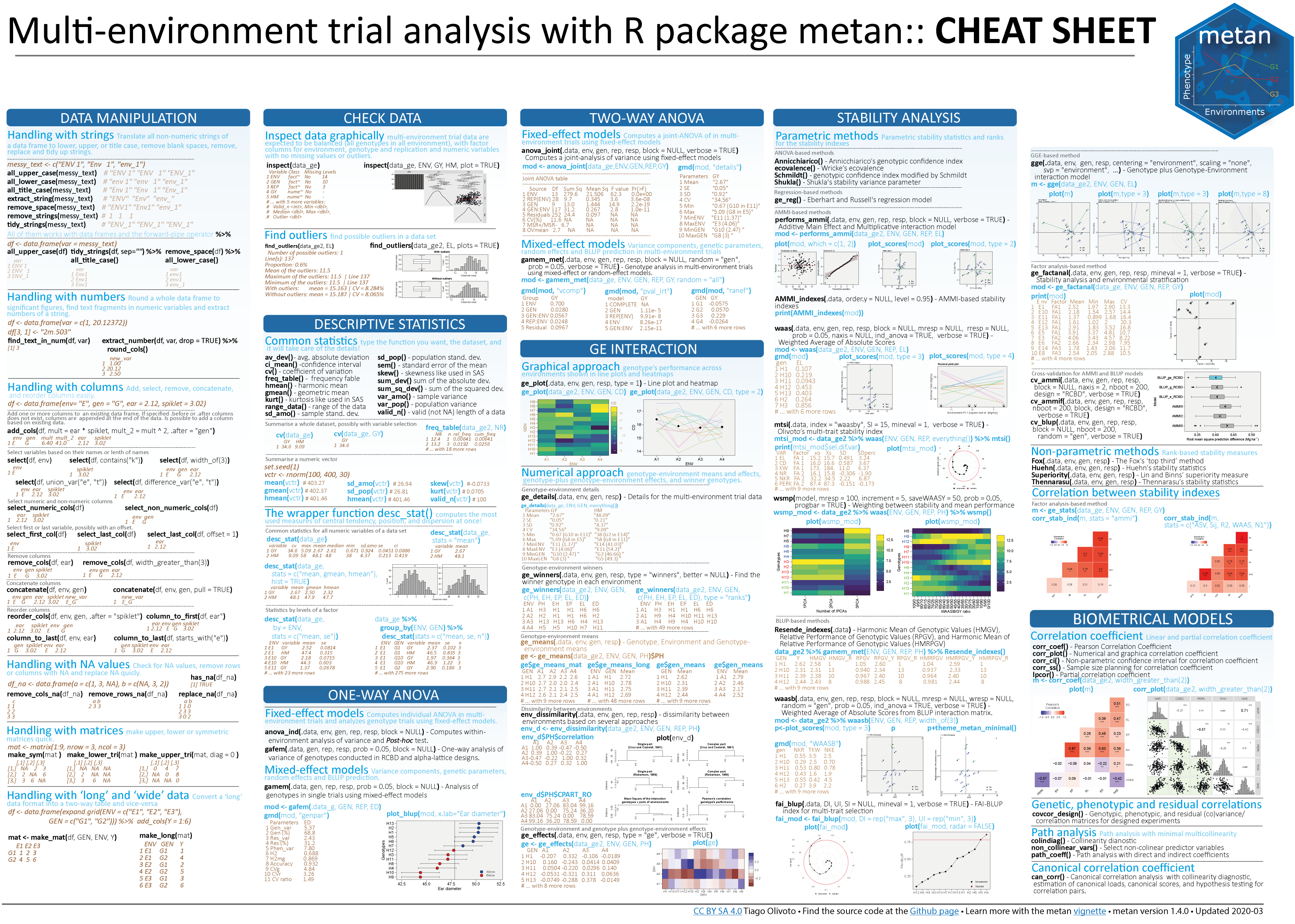
Cheatsheet
Citation
To cite metan in your publications, please, use the official reference paper:
Olivoto, T., and Lúcio, A.D. (2020). metan: an R package for multi-environment trial analysis. Methods Ecol Evol. 11:783-789 doi: 10.1111/2041-210X.13384
A BibTeX entry for LaTeX users is
@Article{Olivoto2020,
    author = {Tiago Olivoto and Alessandro Dal'Col L{'{u}}cio},
    title = {metan: an R package for multi-environment trial analysis},
    journal = {Methods in Ecology and Evolution},
    volume = {11},
    number = {6},
    pages = {783-789},
    year = {2020},
    doi = {10.1111/2041-210X.13384},
  }