Toward an effective multivariate selection in biological experiments
Este post também pode ser lido em Português
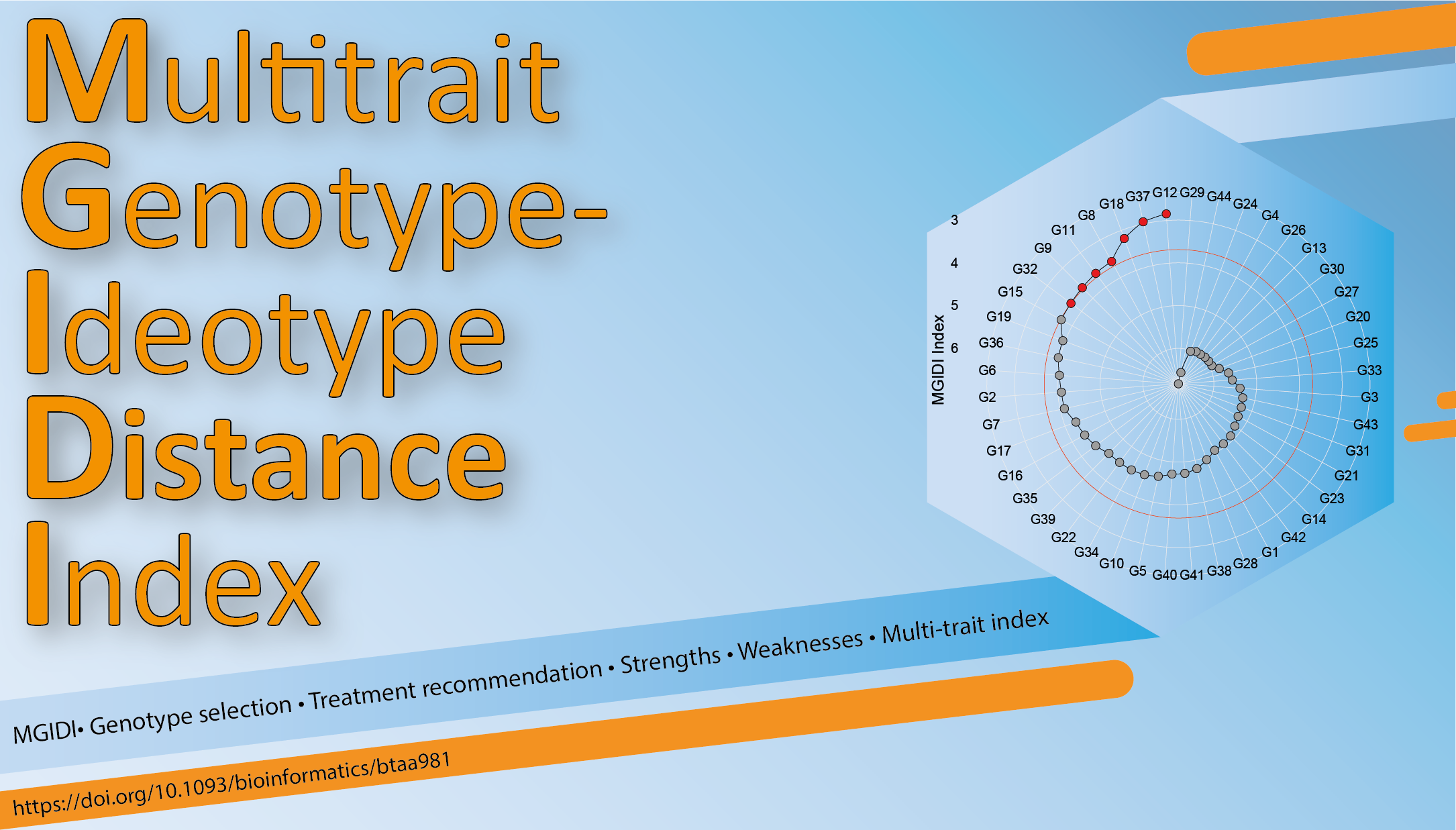
In our recent paper in Bioinformatics, Maicon Nardino and I describe a new multi-trait genotype-ideotype distance index, MGIDI, for genotype selection and treatment recommendation in biological experiments. So, I prepared this short tutorial on the MGIDI computation.
Motivation
Nardino and I have been working with multi-trait data since I started my Mastership at the Federal University of Santa Maria (about five years ago), and selecting genotypes based on multiple traits was always in our radar.
Multivariate data are common in biological experiments and using the information on multiple traits is crucial to make better decisions for treatment recommendations or genotype selection. Classical linear multi-trait selection indexes such as Smith and Hazel index are available, but the presence of multicollinearity and the arbitrary choosing of weighting coefficients may erode the genetic gains.
After one of my Doctoral thesis chapter has been published as “Mean Performance and Stability in Multi‐Environment Trials II: Selection Based on Multiple Traits” I was convinced that combining factor analysis and Euclidean distance principles would be a good strategy for creating a multi-trait index for genotype selection in which most of the characteristics are selected favorably. I also need to thank my Doctoral advisor, Alessandro Dal’Col Lúcio for all the support and partnership and all Graduate and Post-graduate colleagues at that time. At that time (2019) Nardino was alredy Professor in Genetics and Breeding at Federal University of Viçosa and I Professor of Agronomy At Centro Univesitario UNIDEAU. After a lot of long Skype calls, we had the theoretical fundations of the MGIDI index.
Theoretical fundations
The theory behind MGIDI index is centered on four main steps.
-
Rescaling the traits so that all have a 0-100 range
-
Using factor analysis to account for the correlation structure and dimensionality reduction of data.
-
Planning an ideotype based on known/desired values of traits.
-
To compute the distance between each genotype to the planned ideotype.
The genotype/treatment with the lowest MGIDI is then closer to the ideotype and therefore presents desired values for all the p traits.
Software implementation
metan R package has been spread among breeders. So, it seemed logical that there was no other way to provide freely and open-source acessebility of the MGIDI index than implementing it on
metan. An here we’re! the MGIDI index can be computed with metan::mgidi().
The latest stable version of metan is on CRAN and can be obtained with
# The latest stable version is installed with
install.packages("metan")

# Or the development version from GitHub:
# install.packages("devtools")
devtools::install_github("TiagoOlivoto/metan")
Users can fit the index either using replicate-based data or mean-based data.
Using replicate-based data
When replicate-based data are available, both mixed- or fixed-effect models can be fitted with gamem() and gafem(), respectively. In this motivating example, we will reproduce the results for the wheat genotype selection performed in our paper
The first step is to compute the model. In this case, a mixed-effect model with genotype as random effect.
library(metan)
# Registered S3 method overwritten by 'GGally':
#   method from
#   +.gg   ggplot2
# |=========================================================|
# | Multi-Environment Trial Analysis (metan) v1.15.0        |
# | Author: Tiago Olivoto                                   |
# | Type 'citation('metan')' to know how to cite metan      |
# | Type 'vignette('metan_start')' for a short tutorial     |
# | Visit 'https://bit.ly/pkgmetan' for a complete tutorial |
# |=========================================================|
data <-
  read.csv("https://bit.ly/2Z0A7FL", sep = ";") %>%
  as_factor(GEN, BLOCK)

# Fit the mixed-effect model
mod <- gamem(data,
             gen = GEN,
             rep = BLOCK,
             resp = everything(),
             verbose = FALSE)
After fitting the mixed model, we use it as input data in the function mgidi(). In this case, our aim was to select genotypes with negative gains for the first four traits in data and positive gains for the last 10 traits.
mgidi_index <-
  mgidi(mod,
        ideotype = c(rep("l", 4), rep("h", 10)),
        SI = 15,
        verbose = FALSE)
gmd(mgidi_index) %>% round_cols()
# Class of the model: mgidi
# Variable extracted: sel_dif
# # A tibble: 14 x 11
#    VAR   Factor      Xo      Xs     SD SDperc    h2     SG SGperc sense     goal
#    <chr> <chr>    <dbl>   <dbl>  <dbl>  <dbl> <dbl>  <dbl>  <dbl> <chr>    <dbl>
#  1 NSS   FA1      15.5    16.0    0.45   2.9   0.77   0.34   2.22 increase   100
#  2 SL    FA1       8.63    9.12   0.5    5.78  0.67   0.33   3.86 increase   100
#  3 SW    FA1       2.17    2.54   0.37  17.1   0.84   0.31  14.3  increase   100
#  4 NGS   FA1      40.5    42.0    1.51   3.73  0.65   0.99   2.45 increase   100
#  5 GMS   FA1       1.62    1.88   0.26  16.0   0.81   0.21  13.0  increase   100
#  6 HW    FA2      76.3    77.7    1.37   1.79  0.8    1.1    1.44 increase   100
#  7 HIS   FA2      74.7    74.2   -0.52  -0.7   0.79  -0.41  -0.55 increase     0
#  8 PH    FA3      86.5    86.4   -0.08  -0.09  0.78  -0.06  -0.07 decrease   100
#  9 SH    FA3      77.8    77.1   -0.7   -0.9   0.82  -0.57  -0.74 decrease   100
# 10 FLH   FA3      60.4    58.7   -1.68  -2.78  0.83  -1.39  -2.29 decrease   100
# 11 FLO   FA4      60.4    59.1   -1.34  -2.22  0.92  -1.24  -2.05 decrease   100
# 12 DIS   FA4       2.84    3.11   0.27   9.53  0.9    0.24   8.54 increase   100
# 13 NGSP  FA4       2.62    2.64   0.02   0.9   0.52   0.01   0.46 increase   100
# 14 GY    FA5    4380.   4621.   241.     5.5   0.72 173.     3.96 increase   100
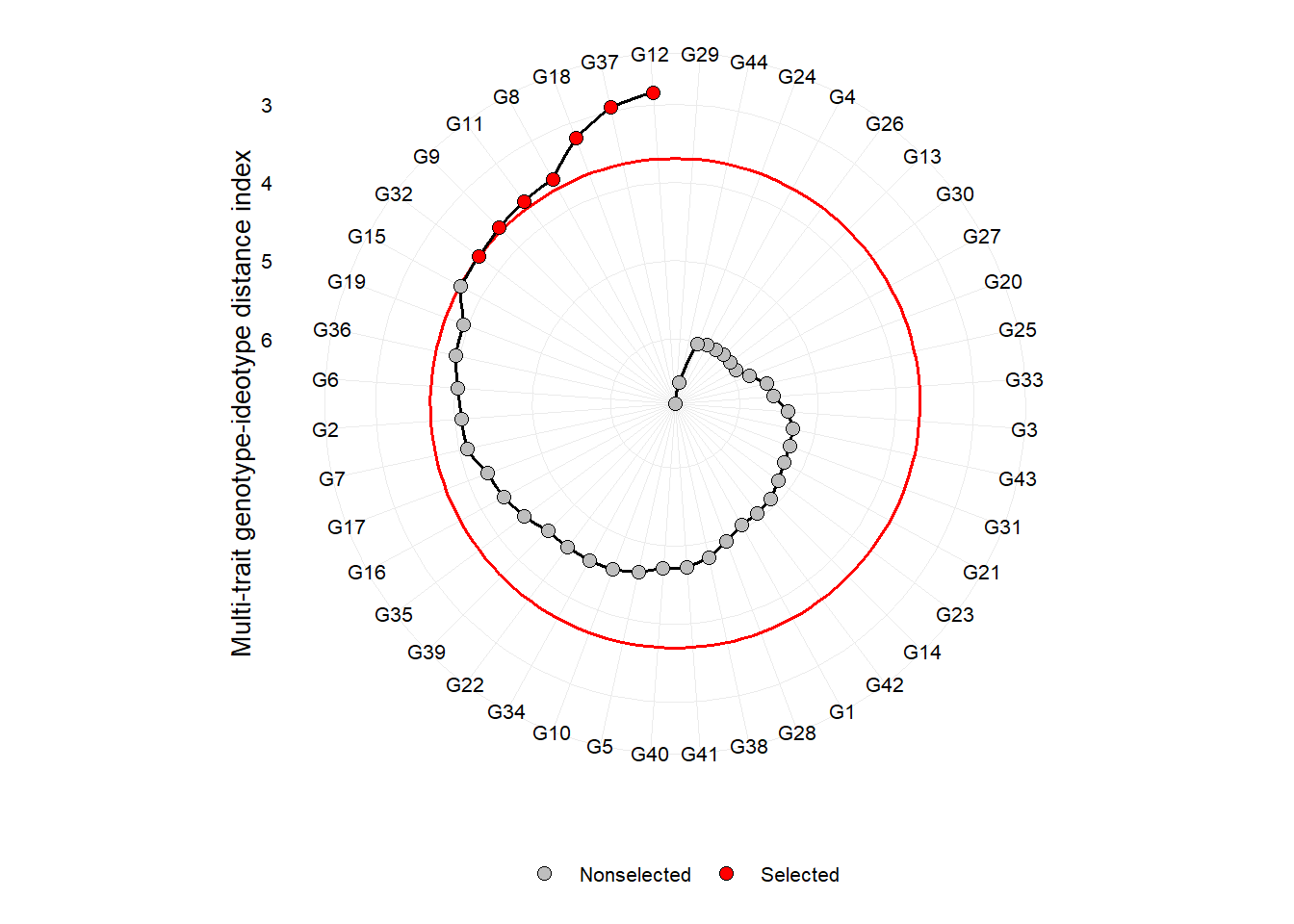
Then, we obtain the genotype/treatment ranking with
plot(mgidi_index)
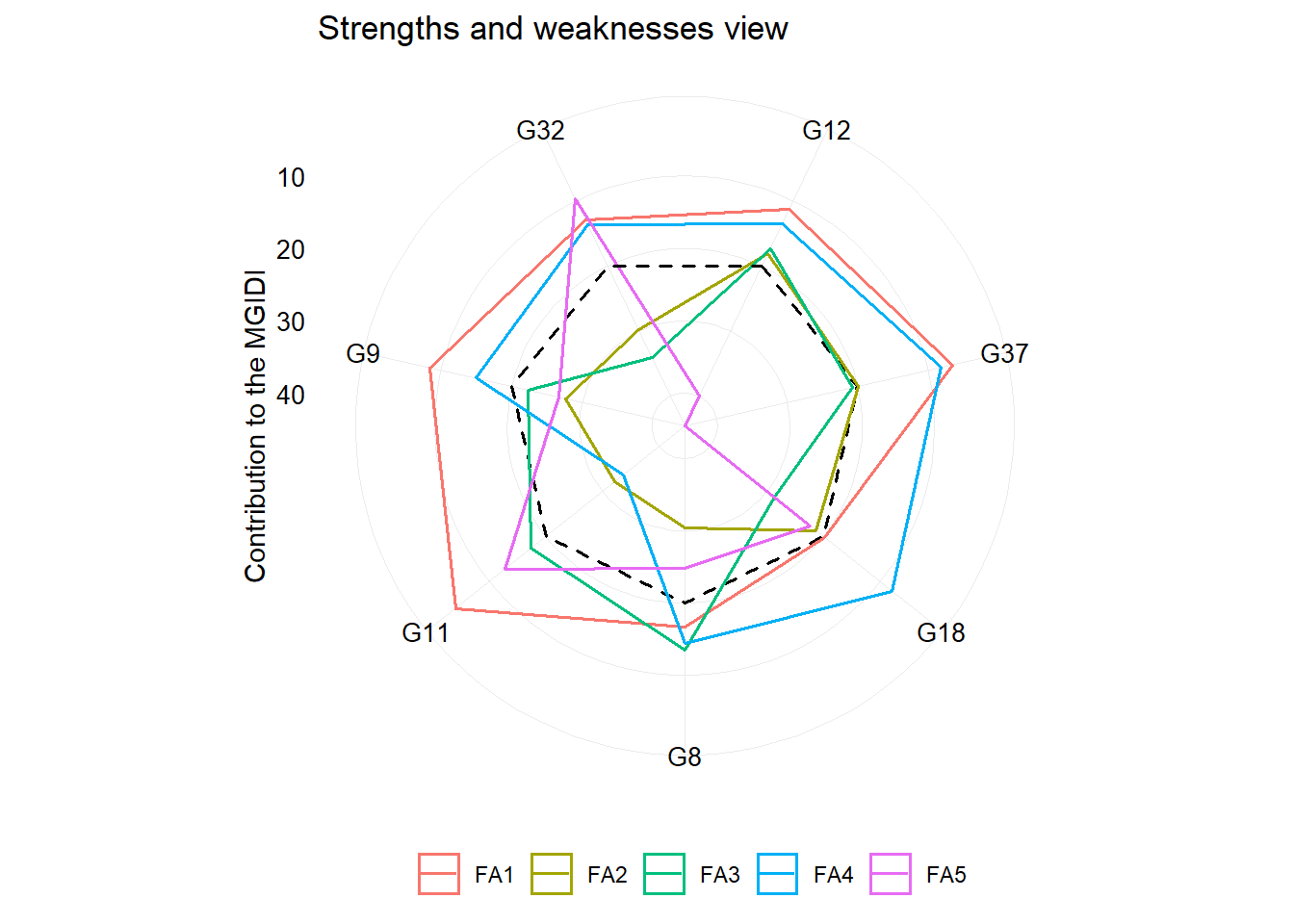
One of the main differentials of MGIDI index is the strengths and weaknesses view of genotypes/treatments using the following radar plot. The factor with the smallest contribution will be closer to the edge of the radar; then the genotype that stands out for this factor will have strengths related to the traits within that factor.
plot(mgidi_index, type = "contribution")
Using a two-way table data
In this section, we extend the theory of the MGIDI index to evaluate an experiment (
Olivoto et al., 2016) with a two-way qualitative-qualitative treatment structure. The focus is to choose the best treatment that allows desired values for most of the evaluated traits. Here, the goal is to obtain low value for P and PL and high values for the remaining traits. Note that the input needed in the function mgidi() is a two-way table with treatment/genotypes in the row names and traits in the columns.
data_ns <-
   read.csv("https://bit.ly/3jKx8Jo", sep = ";")
   str(data_ns)
# 'data.frame':	8 obs. of  11 variables:
#  $ TRAT: chr  "WS_100DR" "WS_30T_40DR_30B" "WS_50T_50DR" "WS_50DR_50B" ...
#  $ P   : num  91.5 96.8 93.5 96.8 103.5 ...
#  $ PL  : num  0.99 1.14 1.32 1.12 1.31 1.1 1.38 1.29
#  $ L   : num  93.2 85.2 71.5 86.8 79 ...
#  $ TIL : num  3.56 5.48 6.55 4.47 3.53 5.42 5.33 4.42
#  $ SSM : num  582 794 702 626 550 ...
#  $ GY  : num  5301 6459 6079 5697 5485 ...
#  $ HW  : num  79.2 79.2 79.2 79.5 78.8 ...
#  $ W   : num  261 264 224 263 270 ...
#  $ GLU : num  30.1 29.9 27.9 29.6 27.6 ...
#  $ PROT: num  11.8 11.9 12.6 12.6 12.7 ...

data_mat <-
  column_to_rownames(data_ns, "TRAT")
# Define the ideotype vector
ide_vect <- c("l", "l", rep("h", 8))
ide_vect
#  [1] "l" "l" "h" "h" "h" "h" "h" "h" "h" "h"


mgidi_data_ns <-
  mgidi(data_mat,
        ideotype = ide_vect,
        verbose = FALSE)
gmd(mgidi_data_ns) %>% round_cols()
# Class of the model: mgidi
# Variable extracted: sel_dif
# # A tibble: 10 x 8
#    VAR   Factor      Xo      Xs     SD SDperc sense     goal
#    <chr> <chr>    <dbl>   <dbl>  <dbl>  <dbl> <chr>    <dbl>
#  1 PL    FA1       1.21    1.14  -0.07  -5.49 decrease   100
#  2 L     FA1      81.7    85.2    3.59   4.4  increase   100
#  3 HW    FA1      79.2    79.2    0.03   0.04 increase   100
#  4 GLU   FA1      28.7    29.8    1.12   3.91 increase   100
#  5 PROT  FA1      12.3    11.9   -0.4   -3.28 increase     0
#  6 P     FA2      97.2    96.8   -0.47  -0.48 decrease   100
#  7 W     FA2     256.    264.     7.78   3.04 increase   100
#  8 TIL   FA3       4.84    5.48   0.64  13.1  increase   100
#  9 SSM   FA3     663.    794.   132.    19.9  increase   100
# 10 GY    FA3    5941.   6459    518.     8.73 increase   100
The MGIDI index indicated the treatment WS_30T_40DR_30B (30% N at the tillering stage, 40% N at the double ring stage, and 30% N at the boosting stage with sulfur implementation) as the best performing treatment. This treatment provides desired values (lower or higher value) for 9 of the 10 analyzed traits, thus, the success rate, in this case, was 90%.
The MGIDI in practice
The MGIDI index allows a unique and easy-to-interpret selection process. Besides dealing with collinear traits, the MGIDI index doesn’t require the use of any economic weights, providing more balanced gains. This means that the MGIDI index can help breeders to guarantee long-term gains in primary traits (e.g., grain yield) without jeopardizing genetic gains of secondary traits (e.g., plant height).
Our
Supplementary data provides the codes used in our article that can be easily adapted in future studies. Another useful function of the metan package that can facilitate the implementation of the multi-trait indexes in future studies is coincidence_index(), which will make it easier for comparing MGIDI, Smith-Hazel and FAI-BLUP indexes in future studies.
Follow our
paper on Research Gate.
Share this post in your social media.
Enjoy MGIDI index.