metan v1.7.0 now on CRAN
I’m so excited to announce that the latest stable version (v1.7.0) of the R package metan is now on
CRAN. The main features included in this version are detailed below.
- New function
sum_by()to compute the sum by levels of factors
library(metan)
# Registered S3 method overwritten by 'GGally':
#   method from
#   +.gg   ggplot2
# []=====================================================[]
# [] Multi-Environment Trial Analysis (metan) v1.7.0     []
# [] Author: Tiago Olivoto                               []
# [] Type citation('metan') to know how to cite metan    []
# [] Type vignette('metan_start') for a short tutorial   []
# [] Visit http://bit.ly/2TIq6JE for a complete tutorial []
# []=====================================================[]
sum_by(data_ge, GEN)
# # A tibble: 10 x 3
#    GEN      GY    HM
#    <fct> <dbl> <dbl>
#  1 G1     109. 1977.
#  2 G10    104. 2037.
#  3 G2     115. 1960.
#  4 G3     124. 1999.
#  5 G4     111. 2017.
#  6 G5     107. 2070.
#  7 G6     106. 2047.
#  8 G7     115. 2015.
#  9 G8     126. 2062.
# 10 G9     105. 2012.
mgidi()now allows using a fixed-effect model fitted withgafem()as input data.
model <- gafem(data_g,
gen = GEN,
rep = REP,
resp = c(NR, KW, CW, CL, NKE, TKW, PERK, PH),
verbose = FALSE)
# Selection for increase all variables
mgidi_model <- mgidi(model)
#
# -------------------------------------------------------------------------------
# Principal Component Analysis
# -------------------------------------------------------------------------------
# # A tibble: 8 x 4
# PC Eigenvalues `Variance (%)` `Cum. variance (%)`
# <chr> <dbl> <dbl> <dbl>
# 1 PC1 3.89 48.6 48.6
# 2 PC2 3.09 38.6 87.1
# 3 PC3 0.52 6.48 93.6
# 4 PC4 0.27 3.4 97.0
# 5 PC5 0.18 2.23 99.2
# 6 PC6 0.06 0.7 100.
# 7 PC7 0 0.04 100.
# 8 PC8 0 0.01 100
# -------------------------------------------------------------------------------
# Factor Analysis - factorial loadings after rotation-
# -------------------------------------------------------------------------------
# # A tibble: 8 x 5
# VAR FA1 FA2 Communality Uniquenesses
# <chr> <dbl> <dbl> <dbl> <dbl>
# 1 NR -0.07 -0.9 0.81 0.19
# 2 KW -0.44 -0.84 0.91 0.09
# 3 CW -0.94 -0.28 0.95 0.05
# 4 CL -0.95 0.03 0.91 0.09
# 5 NKE 0.41 -0.85 0.89 0.11
# 6 TKW -0.91 0 0.83 0.17
# 7 PERK 0.93 -0.15 0.89 0.11
# 8 PH 0.02 -0.88 0.77 0.23
# -------------------------------------------------------------------------------
# Comunalit Mean: 0.8713971
# -------------------------------------------------------------------------------
# Selection differential
# -------------------------------------------------------------------------------
# # A tibble: 8 x 10
# VAR Factor Xo Xs SD SDperc h2 SG SGperc sense
# <chr> <chr> <dbl> <dbl> <dbl> <dbl> <dbl> <dbl> <dbl> <chr>
# 1 CW FA 1 20.8 24.1 3.35 16.1 0.880 2.95 14.2 increase
# 2 CL FA 1 28.4 28.8 0.333 1.17 0.901 0.300 1.06 increase
# 3 TKW FA 1 318. 313. -5.16 -1.62 0.712 -3.67 -1.16 increase
# 4 PERK FA 1 87.6 87.6 -0.0643 -0.0733 0.916 -0.0589 -0.0672 increase
# 5 NR FA 2 15.8 18 2.22 14.0 0.736 1.63 10.3 increase
# 6 KW FA 2 147. 171. 24.5 16.7 0.659 16.2 11.0 increase
# 7 NKE FA 2 468. 558. 89.8 19.2 0.713 64.0 13.7 increase
# 8 PH FA 2 2.17 2.35 0.180 8.31 0.610 0.110 5.07 increase
# ------------------------------------------------------------------------------
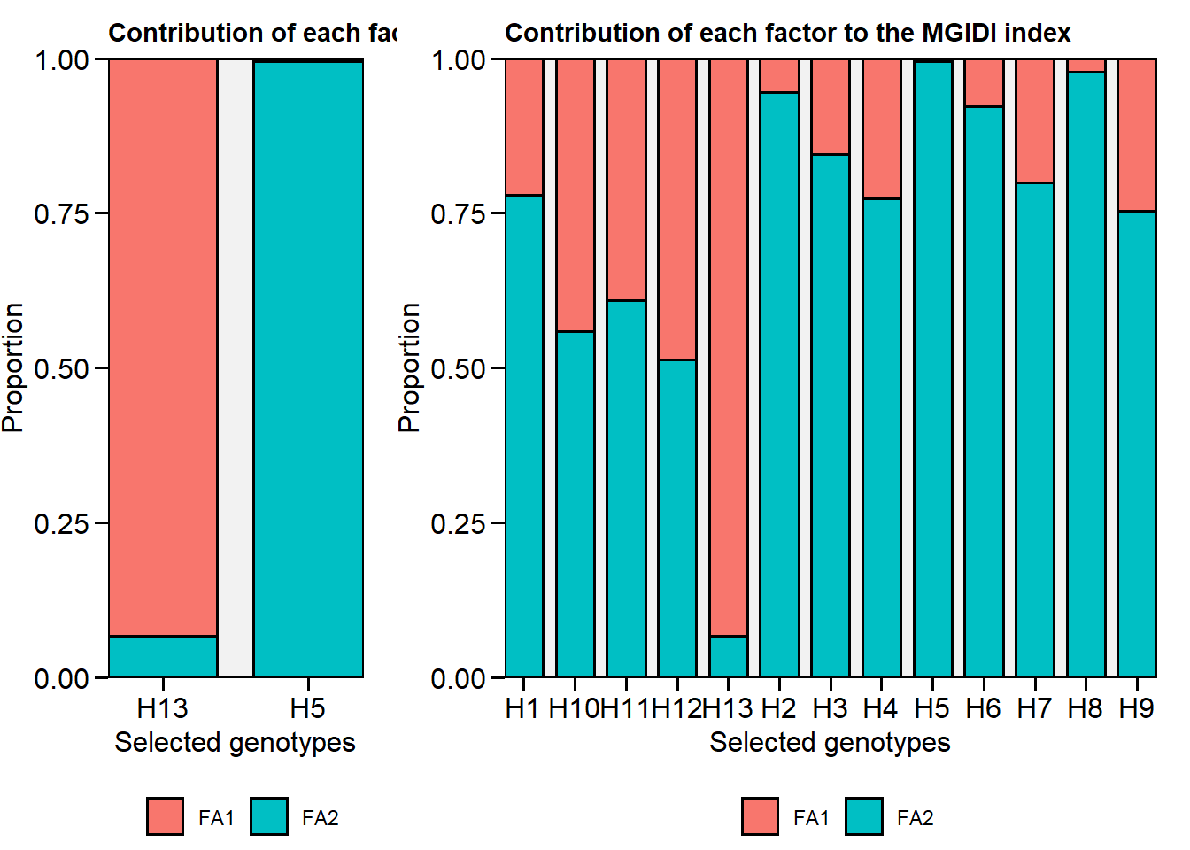
# Selected genotypes
# -------------------------------------------------------------------------------
# H13 H5
# -------------------------------------------------------------------------------
# plot the contribution of each factor on the MGIDI index
p1 <- plot(mgidi_model, type = "contribution")
p2 <- plot(mgidi_model, type = "contribution", genotypes = "all")
arrange_ggplot(p1, p2, rel_widths = c(1, 2))
round_cols()now can be used to round whole matrices.
corr <- corr_coef(data_ge, verbose = FALSE)$cor
corr
#           GY        HM
# GY 1.0000000 0.1928171
# HM 0.1928171 1.0000000
round_cols(corr)
#      GY   HM
# GY 1.00 0.19
# HM 0.19 1.00
- New functions
clip_read()andclip_write()to read from the clipboard and write to the clipboard, respectively. Take a look at the short video bellow to see how them work!
citation("metan")
#
# Please, support this project by citing it in your publications!
#
#   Olivoto, T., and Lúcio, A.D. (2020). metan: an R package for
#   multi-environment trial analysis. Methods Ecol Evol. 11:783-789
#   doi:10.1111/2041-210X.13384
#
# A BibTeX entry for LaTeX users is
#
#   @Article{Olivoto2020,
#     author = {Tiago Olivoto and Alessandro Dal'Col L{'{u}}cio},
#     title = {metan: an R package for multi-environment trial analysis},
#     journal = {Methods in Ecology and Evolution},
#     volume = {11},
#     number = {6},
#     pages = {783-789},
#     year = {2020},
#     doi = {10.1111/2041-210X.13384},
#     url = {https://besjournals.onlinelibrary.wiley.com/doi/abs/10.1111/2041-210X.13384},
#     eprint = {https://besjournals.onlinelibrary.wiley.com/doi/pdf/10.1111/2041-210X.13384},
#   }
Follow metan on Github to find out the latest news!