Este post também está disponível em Português

Introduction

I am pleased to announce the release of pliman (plant image analysis) 0.2.0 on CRAN. pliman is a package for image analysis, with a special focus on plant images. Image analysis is a useful tool for obtaining quantitative information for target objects. In the context of plant images, quantifying the leaf area, the severity of diseases, the number of lesions, counting the number of grains, obtaining grain statistics (e.g., length and width) are some of the tasks that agronomists, breeders, phytopathologists, geneticists and biologists make routinely.

The package will help you to:

• Measure leaf area with leaf_area()
• Measure disease severity with symptomatic_area()
• Count the number of lesions with count_lesions()
• Count objects in an image with count_objects()
• Get the RGB values for each object in an image with objects_rgb()
• Get object measures with get_measures()
• Plot object measures with plot_measures()

Installation

Install the latest stable version of pliman from CRAN with:

install.packages("pliman")

The development version of pliman can be installed from GitHub with:

devtools::install_github("TiagoOlivoto/pliman")

# To build the HTML vignette use
devtools::install_github("TiagoOlivoto/pliman", build_vignettes = TRUE)

Note: If you are a Windows user, you should also first download and install the latest version of Rtools.

Brief examples

Leaf area

Measuring the leaf area is a very common task for breeders and agronomists. The leaf area is used as a key feature for calculating various indexes, such as the Leaf Area Index (IAF), which quantifies the amount of leaf material in a canopy. In pliman, researchers can measure leaf area using images of leaves in two main ways. The first, using leaf_area() uses a sample of leaves along with a template with a known area. The background, leaf, and template color palettes must be declared. An alternative way of calculating the leaf area in pliman is usingcount_objects(). This function has the advantage of using image segmentation based on various indexes (for example, values of red, green, and blue, RGB). Therefore, the sample palettes do not need to be entered. In the following example, we will calculate the leaf area of the leaves image with this last approach. For more details and other examples, see this vignette.

library(pliman)
# |========================================================|
# | Tools for Plant Image Analysis (pliman 0.2.0)          |
# | Author: Tiago Olivoto                                  |
# | Type 'vignette('pliman_start')' for a short tutorial   |
# | Visit 'https://bit.ly/3eL0dF3' for a complete tutorial |
# |========================================================|
leaves <- image_import(image_pliman("la_leaves.JPG"))
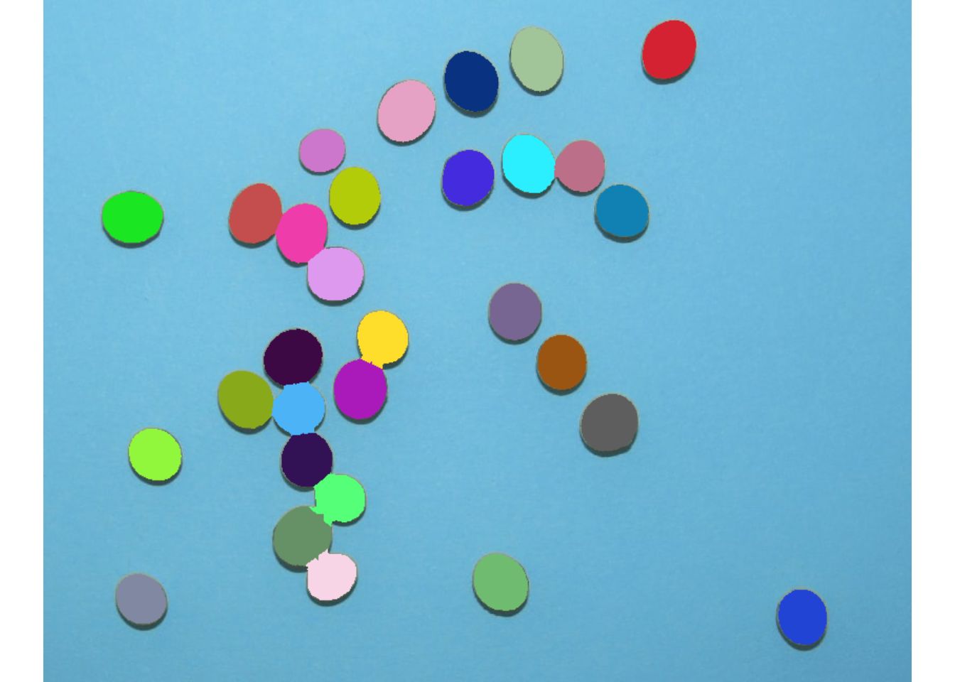
image_show(leaves)

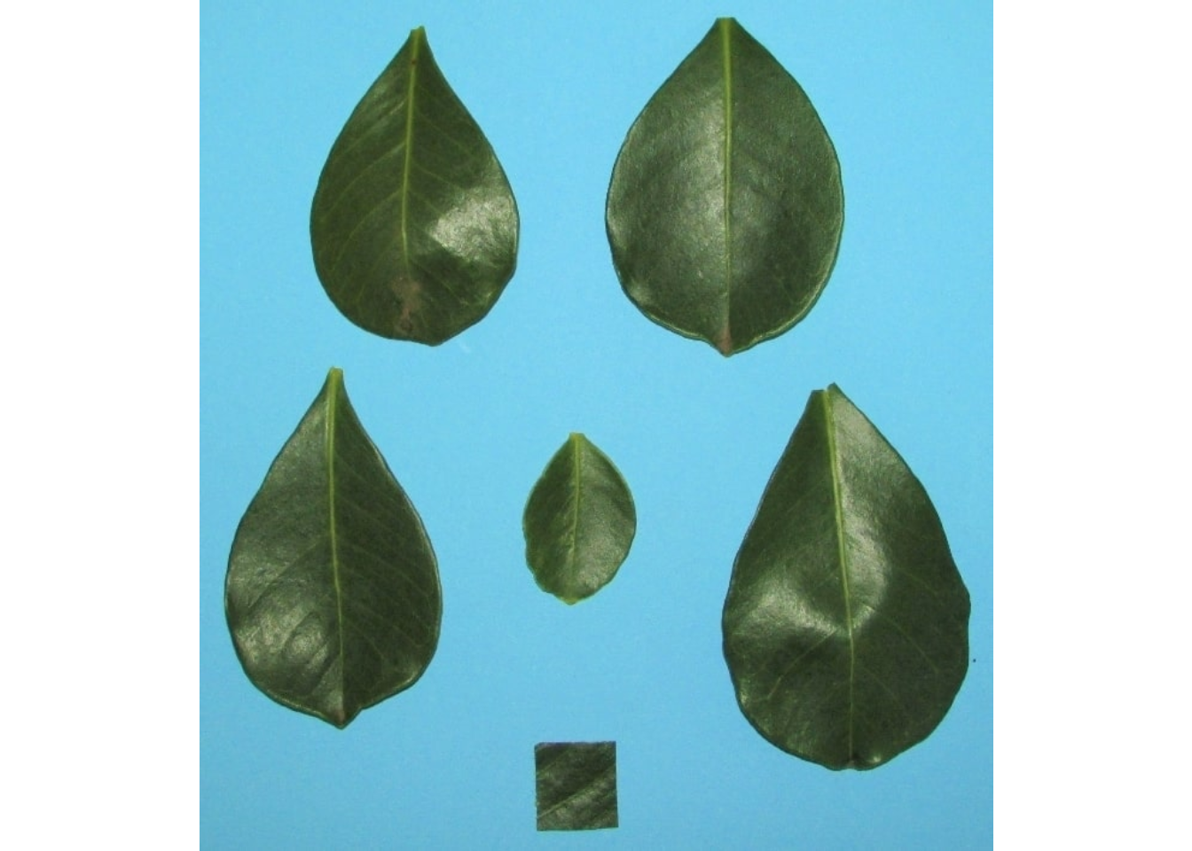
count <- count_objects(leaves)
# 
# --------------------------------------------
# Number of objects: 6 
# --------------------------------------------
#  statistics      area perimeter
#         min   4332.00  253.0000
#        mean  26704.17  533.5000
#         max  44763.00  727.0000
#          sd  16286.76  197.2265
#         sum 160225.00 3201.0000
plot_measures(count)

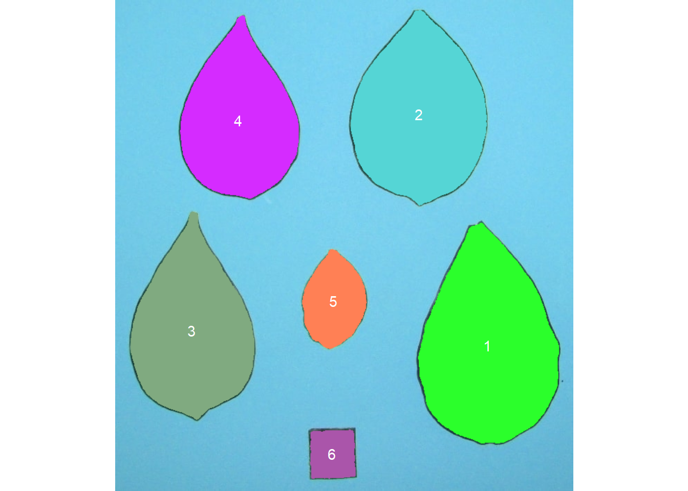
The function get_measures() is used to adjust the leaf area using object 6. It is known that this object has a side of 2 cm, therefore presenting 4 cm$^2$.

area <-
get_measures(count,
             id = 6,
             area ~ 4)
# -----------------------------------------
# measures corrected with:
# object id: 6
# area: 4
# -----------------------------------------
area
#   id        x        y      area perimeter radius_mean radius_min radius_max
# 1  1 537.3833 498.9915 41.332410 22.091245    3.678437   2.756046   5.259454
# 2  2 438.6512 165.2385 35.362881 19.477975    3.370650   2.875019   4.546890
# 3  3 110.8785 477.0276 31.268698 20.116099    3.268759   2.374700   4.856987
# 4  4 178.4196 174.2348 27.445983 18.201727    3.027071   2.307497   4.394600
# 5  5 315.2358 434.6106  8.535549  9.693407    1.655947   1.311698   2.253471
# 6  6 313.4910 655.2052  4.000000  7.687875    1.125488   0.926436   1.378890

Counting grains in an image

Here, we will count the grains in the image soybean_touch.png. This image has a cyan background and contains 30 soybean grains touching each other. Visit this post for more details and examples.

soy <- image_import(image_pliman("soybean_touch.jpg"))
image_show(soy)

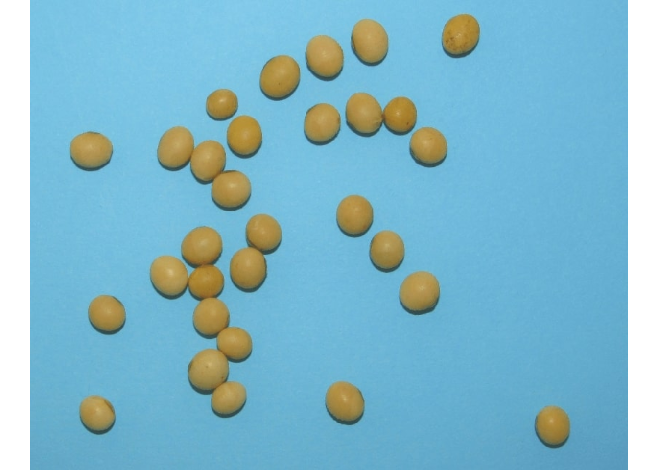
The function count_objects() segments the image using the standard blue index as standard, as follows \(NB = (B / (R + G + B))\), where \(R\), \(G\) and \(B\) are the red, green and blue bands. Objects are counted and segmented objects are colored with random permutations.

count <- count_objects(soy)

# 
# --------------------------------------------
# Number of objects: 30 
# --------------------------------------------
#  statistics       area   perimeter
#         min  1366.0000  117.000000
#        mean  2057.3667  146.600000
#         max  2445.0000  158.000000
#          sd   230.5574    8.406073
#         sum 61721.0000 4398.000000

Users can remove random coloring and identify objects (in this example, grains) using the arguments marker = "text" and show_segmentation = FALSE. The background color can also be changed with col_background argument. In this example, only the five largest grains in area will be identified using topn_upper = 5.

count2 <-
  count_objects(soy,
                marker = "text",
                show_segmentation = FALSE,
                col_background = "white",
                topn_upper = 5)

# 
# --------------------------------------------
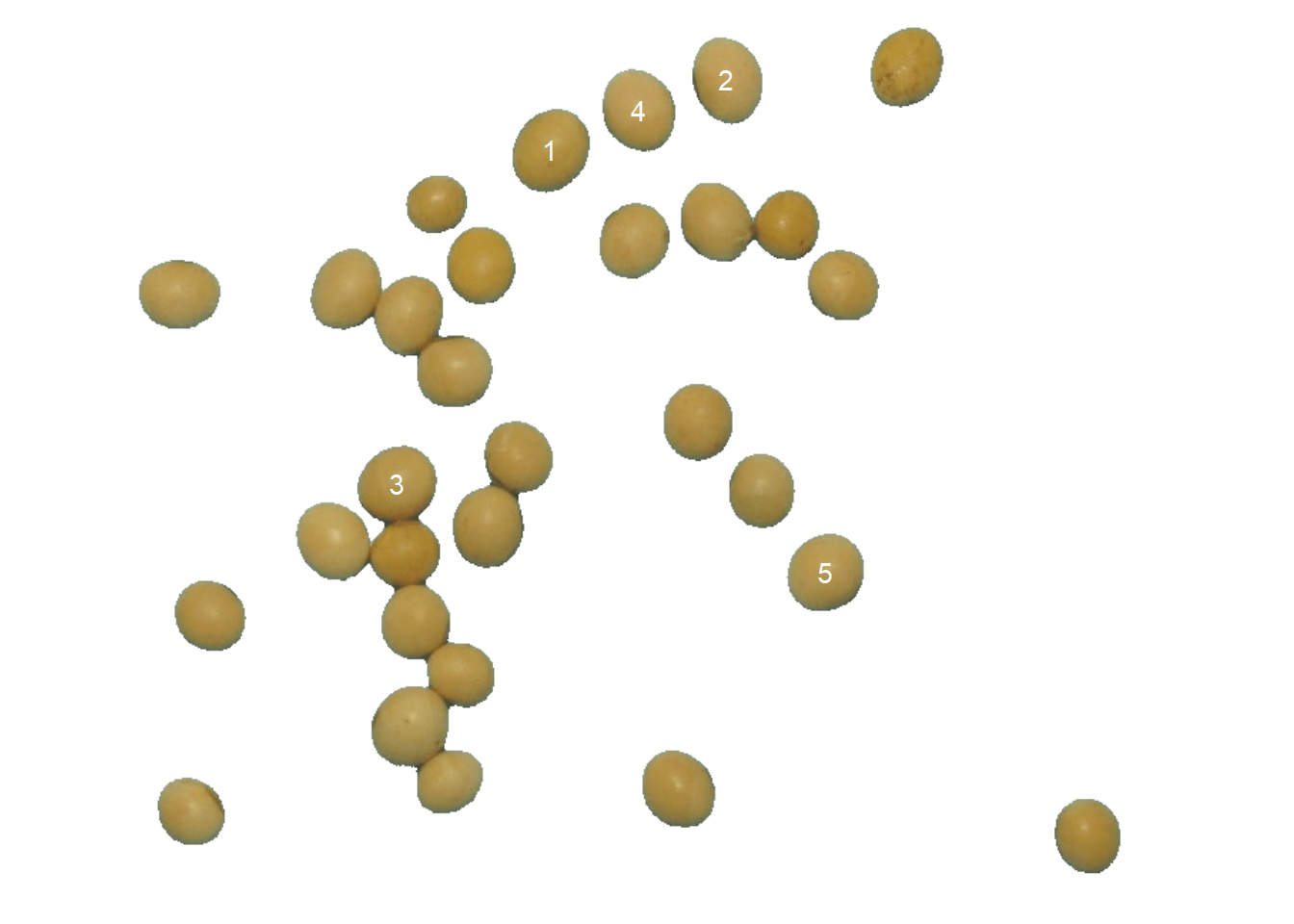
# Number of objects: 5 
# --------------------------------------------
#  statistics        area  perimeter
#         min  2299.00000 152.000000
#        mean  2334.60000 154.200000
#         max  2445.00000 158.000000
#          sd    62.07495   2.387467
#         sum 11673.00000 771.000000


# Get the object measures
(medidas <- get_measures(count2))
#    id        x         y area perimeter radius_mean radius_min radius_max
# 4   1 345.3566 105.78323 2445       158    27.51343   24.68250   30.47116
# 11  2 468.9970  56.42549 2315       155    26.76542   23.03064   30.78003
# 3   3 237.5917 339.82483 2312       152    26.69878   23.96521   29.04402
# 5   4 406.9314  77.54909 2302       153    26.64891   23.96546   29.63586
# 2   5 538.0561 401.89604 2299       153    26.60716   24.95688   28.40020

Disease severity

The disease severity in plants is an important parameter to measure the level of disease and, therefore, can be used to predict production and recommend treatments. In pliman, the function symptomatic_area() is used to quantify the severity of diseases. The user provides color palettes, tells pliman what each one represents and it take care of the details.

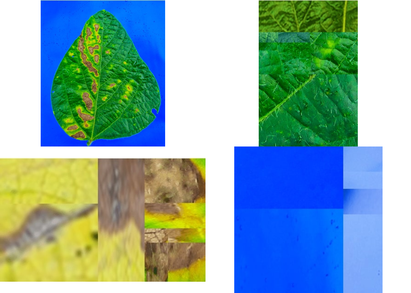
img <- image_import(image_pliman("sev_leaf.jpg"))
healthy <- image_import(image_pliman("sev_healthy.jpg"))
symptoms <- image_import(image_pliman("sev_sympt.jpg"))
background <- image_import(image_pliman("sev_back.jpg"))
image_combine(img, healthy, symptoms,background)

# Compute disease severity
symptomatic_area(img = img,
                 img_healthy = healthy,
                 img_symptoms = symptoms,
                 img_background = background,
                 show_image = TRUE)

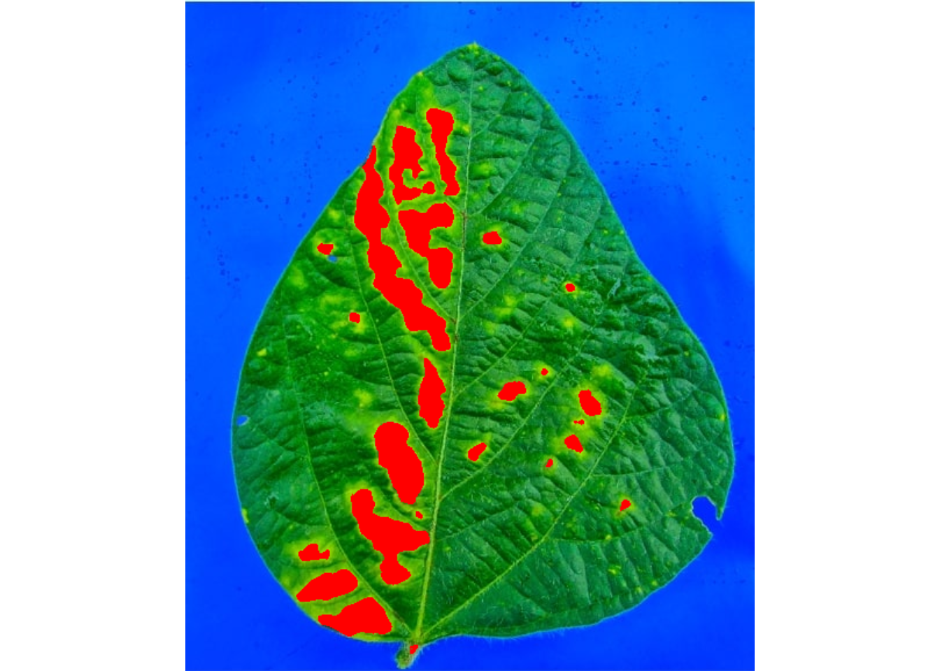
#    healthy symptomatic
# 1 89.10684    10.89316

Batch processing

In plant image analysis, frequently it is necessary to process more than one image. For example, in plant breeding, the number of grains per plant (e.g., wheat) is frequently used in the indirect selection of high-yielding plants. In pliman, batch processing can be done when the user declares the argument img_pattern.

The following example would be used to count the objects in the images with a pattern name "trat" (e.g., "trat1", "trat2", "tratn") saved into the subfolder “originals" in the current working directory. The processed images will be saved into the subfolder "processed". The object list_res will be a list with two objects (results and statistics) for each image.

To speed up the processing time, especially for a large number of images, the argument parallel = TRUE can be used. In this case, the images are processed asynchronously (in parallel) in separate R sessions running in the background on the same machine. The number of sections is set up to 90% of available threads. This number can be controlled explicitly with the argument workers.

list_res <- 
count_objects(img_pattern = "trat", # matches the name pattern in 'originals' subfolder
              dir_original = "originals",
              dir_processed = "processed",
              parallel = TRUE, # parallel processing
              workers = 8, # 8 multiple sections
              save_image = TRUE)

Follow the pliman project in Research Gate.
Share this post on your social networks.
Enjoy the features of the package!