metan v1.10.0 now on CRAN
I’m very pleased to announce that metan 1.10.0 is now on
CRAN. Some minor improvements and new functions were added in this version.
Instalation
# The latest stable version is installed with
install.packages("metan")

# Or the development version from GitHub:
# install.packages("devtools")
devtools::install_github("TiagoOlivoto/metan")
New functions
get_dist()to get distance matrices from objects of classclustering.
library(metan)
# Registered S3 method overwritten by 'GGally':
#   method from
#   +.gg   ggplot2
# |========================================================|
# | Multi-Environment Trial Analysis (metan) v1.11.0       |
# | Author: Tiago Olivoto                                  |
# | Type 'citation('metan')' to know how to cite metan     |
# | Type 'vignette('metan_start')' for a short tutorial    |
# | Visit 'https://bit.ly/2TIq6JE' for a complete tutorial |
# |========================================================|
d <- data_ge2 %>%
      means_by(GEN) %>%
      column_to_rownames("GEN") %>%
      clustering()
get_dist(d)$d %>% round_cols(digits = 1)
#       H1  H10  H11  H12  H13   H2   H3   H4   H5   H6   H7   H8   H9
# H1   0.0 49.2 36.6 55.9 39.8 22.0 28.6 34.5 42.5 10.8 25.0 50.6 63.5
# H10 49.2  0.0 13.7  8.3 43.0 48.9 29.2 46.0 48.1 51.3 26.9  8.8 16.6
# H11 36.6 13.7  0.0 20.0 40.1 40.2 16.2 41.0 45.3 40.2 13.6 14.4 27.1
# H12 55.9  8.3 20.0  0.0 49.1 56.0 34.0 52.9 54.4 58.5 32.7  8.6  9.7
# H13 39.8 43.0 40.1 49.1  0.0 20.8 48.0  9.1  6.8 32.5 40.8 49.9 58.2
# H2  22.0 48.9 40.2 56.0 20.8  0.0 40.9 14.2 22.0 12.7 34.5 53.6 64.9
# H3  28.6 29.2 16.2 34.0 48.0 40.9  0.0 46.8 53.0 36.1  7.9 26.5 39.3
# H4  34.5 46.0 41.0 52.9  9.1 14.2 46.8  0.0  8.7 26.2 39.7 52.5 61.9
# H5  42.5 48.1 45.3 54.4  6.8 22.0 53.0  8.7  0.0 34.1 45.6 55.2 63.3
# H6  10.8 51.3 40.2 58.5 32.5 12.7 36.1 26.2 34.1  0.0 30.9 54.4 66.7
# H7  25.0 26.9 13.6 32.7 40.8 34.5  7.9 39.7 45.6 30.9  0.0 26.2 39.2
# H8  50.6  8.8 14.4  8.6 49.9 53.6 26.5 52.5 55.2 54.4 26.2  0.0 13.2
# H9  63.5 16.6 27.1  9.7 58.2 64.9 39.3 61.9 63.3 66.7 39.2 13.2  0.0
get_corvars()to get normal, multivariate correlated variables.
sigma <- matrix(c(1,  .3,  0,
                  .3,   1, .9,
                  0,   .9,  1),3,3)
mu <- c(6,50,5)

df <- get_corvars(n = 10000, mu = mu, sigma = sigma, seed = 101010)
means_by(df)
# # A tibble: 1 x 3
#      X1    X2    X3
#   <dbl> <dbl> <dbl>
# 1  6.01  50.0  5.00
cor(df)
#             X1        X2          X3
# X1 1.000000000 0.3026515 0.004851063
# X2 0.302651488 1.0000000 0.900604867
# X3 0.004851063 0.9006049 1.000000000
get_covmat()to obtain covariance matrix based on variances and correlation values.
cormat <-
matrix(c(1,  0.9, -0.4,
         0.9,  1,  0.6,
        -0.4, 0.6, 1),
      nrow = 3,
      ncol = 3)
get_covmat(cormat, var =  c(16, 25, 9))
#      V1 V2   V3
# V1 16.0 18 -4.8
# V2 18.0 25  9.0
# V3 -4.8  9  9.0
as_numeric(),as_integer(),as_logical(),as_character(), andas_factor()to coerce variables to specific formats quickly.
library(metan)
library(tibble)
# Warning: package 'tibble' was built under R version 4.0.3
df <-
  tibble(y = rnorm(5),
         x1 = c(1:5),
         x2 = c(TRUE, TRUE, FALSE, FALSE, FALSE),
         x3 = letters[1:5],
         x4 = as.factor(x3))
df
# # A tibble: 5 x 5
#        y    x1 x2    x3    x4
#    <dbl> <int> <lgl> <chr> <fct>
# 1 -1.59      1 TRUE  a     a
# 2 -1.62      2 TRUE  b     b
# 3 -0.751     3 FALSE c     c
# 4  1.13      4 FALSE d     d
# 5  0.472     5 FALSE e     e

# Convert y to integer
as_integer(df, y)
# # A tibble: 5 x 5
#       y    x1 x2    x3    x4
#   <int> <int> <lgl> <chr> <fct>
# 1    -1     1 TRUE  a     a
# 2    -1     2 TRUE  b     b
# 3     0     3 FALSE c     c
# 4     1     4 FALSE d     d
# 5     0     5 FALSE e     e

# convert x3 to factor
as_factor(df, x3)
# # A tibble: 5 x 5
#        y    x1 x2    x3    x4
#    <dbl> <int> <lgl> <fct> <fct>
# 1 -1.59      1 TRUE  a     a
# 2 -1.62      2 TRUE  b     b
# 3 -0.751     3 FALSE c     c
# 4  1.13      4 FALSE d     d
# 5  0.472     5 FALSE e     e

# Convert all columns to character
as_character(df, everything())
# # A tibble: 5 x 5
#   y                  x1    x2    x3    x4
#   <chr>              <chr> <chr> <chr> <chr>
# 1 -1.59386583725876  1     TRUE  a     a
# 2 -1.61771631653143  2     TRUE  b     b
# 3 -0.751337714367338 3     FALSE c     c
# 4 1.13100276654771   4     FALSE d     d
# 5 0.472487882906806  5     FALSE e     e

# Convert x2 to numeric and coerce to a vector
as_numeric(df, x2, .keep = "used", .pull = TRUE)
# [1] 1 1 0 0 0
n_valid(),n_missing(), andn_unique()to count valid, missing, and unique values, respectively.
library(metan)
data_naz <- iris %>%
              group_by(Species) %>%
              doo(~head(., n = 3)) %>%
              as_character(Species)
data_naz
# # A tibble: 9 x 5
#   Species    Sepal.Length Sepal.Width Petal.Length Petal.Width
#   <chr>             <dbl>       <dbl>        <dbl>       <dbl>
# 1 setosa              5.1         3.5          1.4         0.2
# 2 setosa              4.9         3            1.4         0.2
# 3 setosa              4.7         3.2          1.3         0.2
# 4 versicolor          7           3.2          4.7         1.4
# 5 versicolor          6.4         3.2          4.5         1.5
# 6 versicolor          6.9         3.1          4.9         1.5
# 7 virginica           6.3         3.3          6           2.5
# 8 virginica           5.8         2.7          5.1         1.9
# 9 virginica           7.1         3            5.9         2.1
data_naz[c(2:3, 6, 8), c(1:2, 4, 5)] <- NA
n_valid(data_naz)
# Warning: NA values removed to compute the function. Use 'na.rm = TRUE' to
# suppress this warning.

# Warning: NA values removed to compute the function. Use 'na.rm = TRUE' to
# suppress this warning.

# Warning: NA values removed to compute the function. Use 'na.rm = TRUE' to
# suppress this warning.
# # A tibble: 1 x 4
#   Sepal.Length Sepal.Width Petal.Length Petal.Width
#          <int>       <int>        <int>       <int>
# 1            5           9            5           5
n_missing(data_naz, na.rm = TRUE) # na.rm = TRUE to suppress the warning.
# # A tibble: 1 x 5
#   Species Sepal.Length Sepal.Width Petal.Length Petal.Width
#     <int>        <int>       <int>        <int>       <int>
# 1       4            4           0            4           4
n_unique(data_naz, na.rm = TRUE) # na.rm = TRUE to suppress the warning.
# # A tibble: 1 x 5
#   Species Sepal.Length Sepal.Width Petal.Length Petal.Width
#     <int>        <int>       <int>        <int>       <int>
# 1       4            6           6            6           6
env_stratification()to perform environment stratification using factor analysis.
model <-
env_stratification(data_ge,
                   env = ENV,
                   gen = GEN,
                   resp = everything())
gmd(model)
# Class of the model: env_stratification
# Variable extracted: env_strat
# # A tibble: 28 x 7
#    TRAIT ENV   MEGA_ENV  MEAN   MIN   MAX    CV
#    <chr> <chr> <chr>    <dbl> <dbl> <dbl> <dbl>
#  1 GY    E1    ME1       2.52 1.97   2.90 13.3
#  2 GY    E10   ME1       2.18 1.54   2.57 14.4
#  3 GY    E11   ME1       1.37 0.899  1.68 16.4
#  4 GY    E12   ME1       1.61 1.02   2    20.3
#  5 GY    E13   ME1       2.91 1.83   3.52 16.8
#  6 GY    E5    ME1       3.91 3.37   4.81 10.7
#  7 GY    E3    ME2       4.06 3.43   4.57  8.22
#  8 GY    E6    ME2       2.66 2.34   2.98  7.95
#  9 GY    E14   ME3       1.78 1.43   2.06 11.7
# 10 GY    E8    ME3       2.54 2.05   2.88 10.5
# # ... with 18 more rows
gmd(model, "FA")
# Class of the model: env_stratification
# Variable extracted: FA
# # A tibble: 28 x 9
#    TRAIT ENV       FA1     FA2      FA3     FA4     FA5 COMMUNALITY UNIQUENESSES
#    <chr> <chr>   <dbl>   <dbl>    <dbl>   <dbl>   <dbl>       <dbl>        <dbl>
#  1 GY    E1    -0.881   0.327   0.00927 -0.0631  0.274        0.963      0.0369
#  2 GY    E10   -0.942  -0.158  -0.0820   0.113   0.174        0.962      0.0380
#  3 GY    E11   -0.929  -0.233  -0.0336  -0.242   0.110        0.989      0.0111
#  4 GY    E12   -0.848   0.135   0.0263   0.0941  0.241        0.805      0.195
#  5 GY    E13   -0.940   0.108  -0.0842  -0.0637 -0.235        0.961      0.0391
#  6 GY    E14   -0.150  -0.123  -0.916   -0.0872  0.265        0.954      0.0463
#  7 GY    E2    -0.198  -0.0521 -0.126   -0.969   0.0328       0.997      0.00266
#  8 GY    E3    -0.0806  0.910   0.341   -0.0173 -0.110        0.963      0.0370
#  9 GY    E4     0.209   0.543  -0.272   -0.728  -0.120        0.957      0.0433
# 10 GY    E5    -0.777   0.392  -0.269   -0.0470 -0.267        0.904      0.0963
# # ... with 18 more rows
Minor improvements
gamem(),gamem_met(), andwaasb()now have abyargument and understand data passed fromgroup_by. Let’s to compute a mixed model within each environment of datasetdata_ge2and extract the variance components for each model.
model <- gamem(data_ge2,
              gen = GEN,
              rep = REP,
              resp = NR:TKW,
              by = ENV,
              verbose = FALSE)
gmd(model, "vcomp", verbose = FALSE)
# # A tibble: 8 x 7
#   ENV   Group       NR   NKR     CDED  PERK   TKW
#   <fct> <chr>    <dbl> <dbl>    <dbl> <dbl> <dbl>
# 1 A1    GEN      1.14   2.37 0.000821 2.79   513.
# 2 A1    Residual 2.92   6.36 0.000553 2.30  1015.
# 3 A2    GEN      1.14   5.33 0.000781 3.92  2941.
# 4 A2    Residual 0.941  5.86 0.000414 0.575  674.
# 5 A3    GEN      1.18   2.15 0.000956 3.14   841.
# 6 A3    Residual 1.27   7.80 0.000376 0.867 1018.
# 7 A4    GEN      0.375  2.75 0.000133 0.486  291.
# 8 A4    Residual 1.44  11.4  0.000398 0.896  967.
mtsi()andmgidi()now returns the ranks for the contribution of each factor and understand models fitted withgamem()andwaasb()using thebyargument.
mgidi_mod <- mgidi(model,
                   mineval = .1, # force a greater number of factors
                   SI = 40,
                   verbose = FALSE)

gmd(mgidi_mod, verbose = FALSE)
# # A tibble: 20 x 12
#    ENV   VAR   Factor      Xo      Xs       SD SDperc    h2       SG  SGperc
#    <fct> <chr> <chr>    <dbl>   <dbl>    <dbl>  <dbl> <dbl>    <dbl>   <dbl>
#  1 A1    PERK  FA1     87.4    87.3   -0.157   -0.179 0.784 -0.123   -0.140
#  2 A1    NKR   FA2     33.9    34.4    0.507    1.50  0.528  0.268    0.791
#  3 A1    TKW   FA3    360.    365.     4.20     1.17  0.603  2.53     0.703
#  4 A1    NR    FA4     16.9    16.9   -0.0210  -0.124 0.539 -0.0113  -0.0670
#  5 A1    CDED  FA5      0.576   0.583  0.00655  1.14  0.817  0.00535  0.928
#  6 A2    CDED  FA1      0.584   0.586  0.00201  0.345 0.850  0.00171  0.293
#  7 A2    PERK  FA1     87.6    88.7    1.02     1.16  0.953  0.971    1.11
#  8 A2    NKR   FA2     32.3    32.2   -0.0503  -0.156 0.732 -0.0368  -0.114
#  9 A2    NR    FA3     15.8    15.6   -0.153   -0.967 0.784 -0.120   -0.758
# 10 A2    TKW   FA4    334.    331.    -2.66    -0.798 0.929 -2.47    -0.741
# 11 A3    CDED  FA1      0.595   0.588 -0.00680 -1.14  0.884 -0.00601 -1.01
# 12 A3    PERK  FA1     87.6    87.1   -0.577   -0.659 0.916 -0.529   -0.603
# 13 A3    NR    FA2     15.8    16.5    0.708    4.49  0.736  0.521    3.30
# 14 A3    NKR   FA3     30.4    30.7    0.253    0.833 0.452  0.115    0.377
# 15 A3    TKW   FA4    318.    325.     7.41     2.33  0.712  5.28     1.66
# 16 A4    TKW   FA1    343.    347.     4.46     1.30  0.475  2.12     0.618
# 17 A4    PERK  FA2     87.0    87.3    0.265    0.305 0.619  0.164    0.189
# 18 A4    NR    FA3     16.0    16.1    0.120    0.746 0.438  0.0524   0.327
# 19 A4    NKR   FA4     32.5    32.9    0.483    1.49  0.420  0.203    0.625
# 20 A4    CDED  FA5      0.589   0.593  0.00345  0.585 0.500  0.00172  0.293
# # ... with 2 more variables: sense <chr>, goal <dbl>
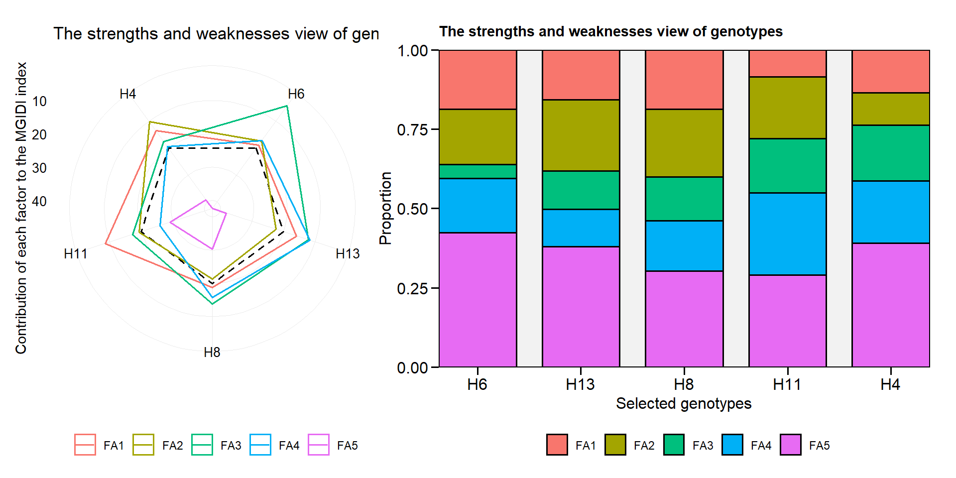
plot.mtsi()andplot.mgidi()now returns a radar plot by default when usingtype = "contribution".
p1 <- plot(mgidi_mod$data[[1]], type = "contribution")
p2 <- plot(mgidi_mod$data[[1]], type = "contribution", radar = FALSE)
arrange_ggplot(p1, p2)
get_model_data()now returns the genotypic and phenotypic correlation matrices from objects of classwaasbandgamem.
(pcor <- gmd(model$data[[1]], "pcor"))
# Class of the model: gamem
# Variable extracted: pcor
#              NR          NKR       CDED         PERK        TKW
# NR    1.0000000 -0.351700402 -0.3271058  0.344913775 -0.4723885
# NKR  -0.3517004  1.000000000 -0.4447736 -0.008091937 -0.1152699
# CDED -0.3271058 -0.444773632  1.0000000 -0.700728407  0.4242704
# PERK  0.3449138 -0.008091937 -0.7007284  1.000000000 -0.2854948
# TKW  -0.4723885 -0.115269899  0.4242704 -0.285494825  1.0000000
(gcor <- gmd(model$data[[1]], "gcor"))
# Class of the model: gamem
# Variable extracted: gcor
#              NR         NKR       CDED        PERK         TKW
# NR    1.0000000 -0.62348035 -0.4359572  0.40578424 -0.37885398
# NKR  -0.6234804  1.00000000 -0.4731984 -0.06763518 -0.07922932
# CDED -0.4359572 -0.47319840  1.0000000 -0.80549808  0.51851366
# PERK  0.4057842 -0.06763518 -0.8054981  1.00000000 -0.32151455
# TKW  -0.3788540 -0.07922932  0.5185137 -0.32151455  1.00000000
- The new function
make_lower_upper()makes it easier to combine two symmetric matrices into one lower-upper diagonal matrix. In the following example, we’ll put the phenotypic correlation matrix in the lower diagonal and the genotypic correlations in the upper diagonal.
make_lower_upper(pcor, gcor, diag = 1)
#              NR          NKR       CDED        PERK         TKW
# NR    1.0000000 -0.623480350 -0.4359572  0.40578424 -0.37885398
# NKR  -0.3517004  1.000000000 -0.4731984 -0.06763518 -0.07922932
# CDED -0.3271058 -0.444773632  1.0000000 -0.80549808  0.51851366
# PERK  0.3449138 -0.008091937 -0.7007284  1.00000000 -0.32151455
# TKW  -0.4723885 -0.115269899  0.4242704 -0.28549482  1.00000000