I’m so proud to announce that metan 1.11.0 is now on CRAN. This minor release include some new functions and minor improvements.

Instalation

# The latest stable version is installed with
install.packages("metan")

# Or the development version from GitHub:
# install.packages("devtools")
devtools::install_github("TiagoOlivoto/metan")

New functions

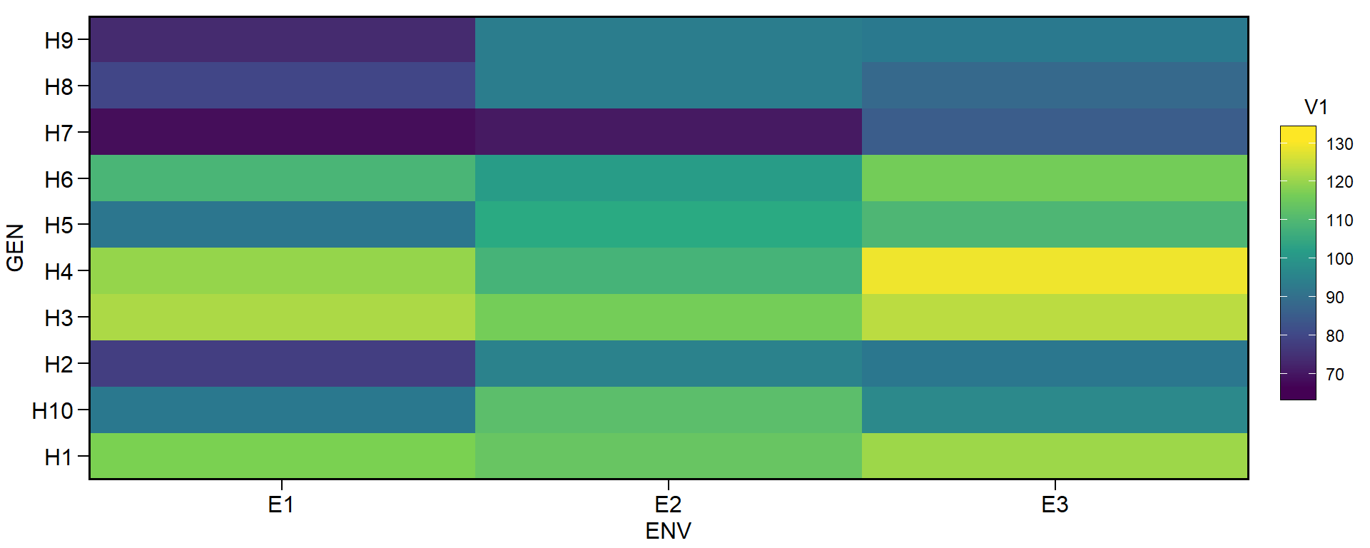
Genotype-environment data

• ge_simula() to simulate genotype-environment data. The function simulates genotype-environment data with different main and interaction effects. The effects are selected from a uniform distribution considering the number of levels of each effect (mandatory arguments) and the effect desired (optional arguments).

library(metan)
# Registered S3 method overwritten by 'GGally':
#   method from   
#   +.gg   ggplot2
# |========================================================|
# | Multi-Environment Trial Analysis (metan) v1.13.0       |
# | Author: Tiago Olivoto                                  |
# | Type 'citation('metan')' to know how to cite metan     |
# | Type 'vignette('metan_start')' for a short tutorial    |
# | Visit 'https://bit.ly/2TIq6JE' for a complete tutorial |
# |========================================================|
df <-
ge_simula(ngen = 10,
          nenv = 3,
          nrep = 4,
          nvars = 2,
          seed = 1:2) # to ensure reproducibility
# Warning: 'gen_eff = 20' recycled for all the 2 traits.
# Warning: 'env_eff = 15' recycled for all the 2 traits.
# Warning: 'rep_eff = 5' recycled for all the 2 traits.
# Warning: 'ge_eff = 10' recycled for all the 2 traits.
# Warning: 'res_eff = 5' recycled for all the 2 traits.
# Warning: 'intercept = 100' recycled for all the 2 traits.
ge_plot(df, ENV, GEN, V1)

# Change genotype effect (trait 1 with fewer differences among genotypes)
# Change environment effect (trait 1 with fewer differences among environments)
# Change interaction effect (trait 1 with fewer interaction effect)
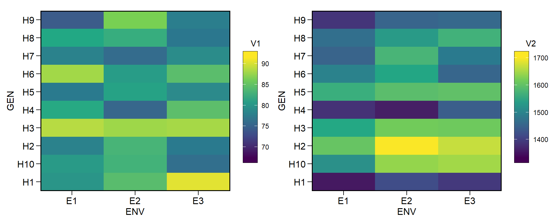
# Define different intercepts for the two traits
df2 <-
ge_simula(ngen = 10,
          nenv = 3,
          nrep = 4,
          nvars = 2,
          gen_eff = c(1, 150),
          env_eff = c(1, 50),
          ge_eff = c(1, 50),
          intercept = c(80, 1500),
          seed = 1:2) # to ensure reproducibility
# Warning: 'rep_eff = 5' recycled for all the 2 traits.
# Warning: 'res_eff = 5' recycled for all the 2 traits.
p1 <- ge_plot(df2, ENV, GEN, V1)
p2 <- ge_plot(df2, ENV, GEN, V2)
p1 + p2

Set operations

Operations with sets are important in the genotype-environment analysis (which metan was designed for). For example, if a genotype was selected by a given index within environments A, B, and C, then, this given genotype is the intersection of environments A, B, and C. R base provides functions for set operations but works with two sets at once only. Let’s see how we could estimate the intersection of three sets with R base functions.

(A <- letters[1:4])
# [1] "a" "b" "c" "d"
(B <- letters[2:5])
# [1] "b" "c" "d" "e"
(C <- letters[3:7])
# [1] "c" "d" "e" "f" "g"
(D <- letters[1:12])
#  [1] "a" "b" "c" "d" "e" "f" "g" "h" "i" "j" "k" "l"
set_lits <- list(A = A, B = B, C = C, D = D)
# intersection of A, B, and C
intersect(intersect(A, B), C)
# [1] "c" "d"

Note that we need call intersect() several times in this case. The new group of functions set_union(), set_difference() and set_intersect() overcomes the problem of computing union, intersection, and differences of two sets only with the R base functions.

# Intersect of A and B
set_intersect(A, B)
# [1] "b" "c" "d"
# Intersect of A, B, and C
set_intersect(A, B, C)
# [1] "c" "d"

# Union of all sets
# All functions understand a list object
set_union(set_lits)
#  [1] "a" "b" "c" "d" "e" "f" "g" "h" "i" "j" "k" "l"
set_intersect(set_lits)
# [1] "c" "d"

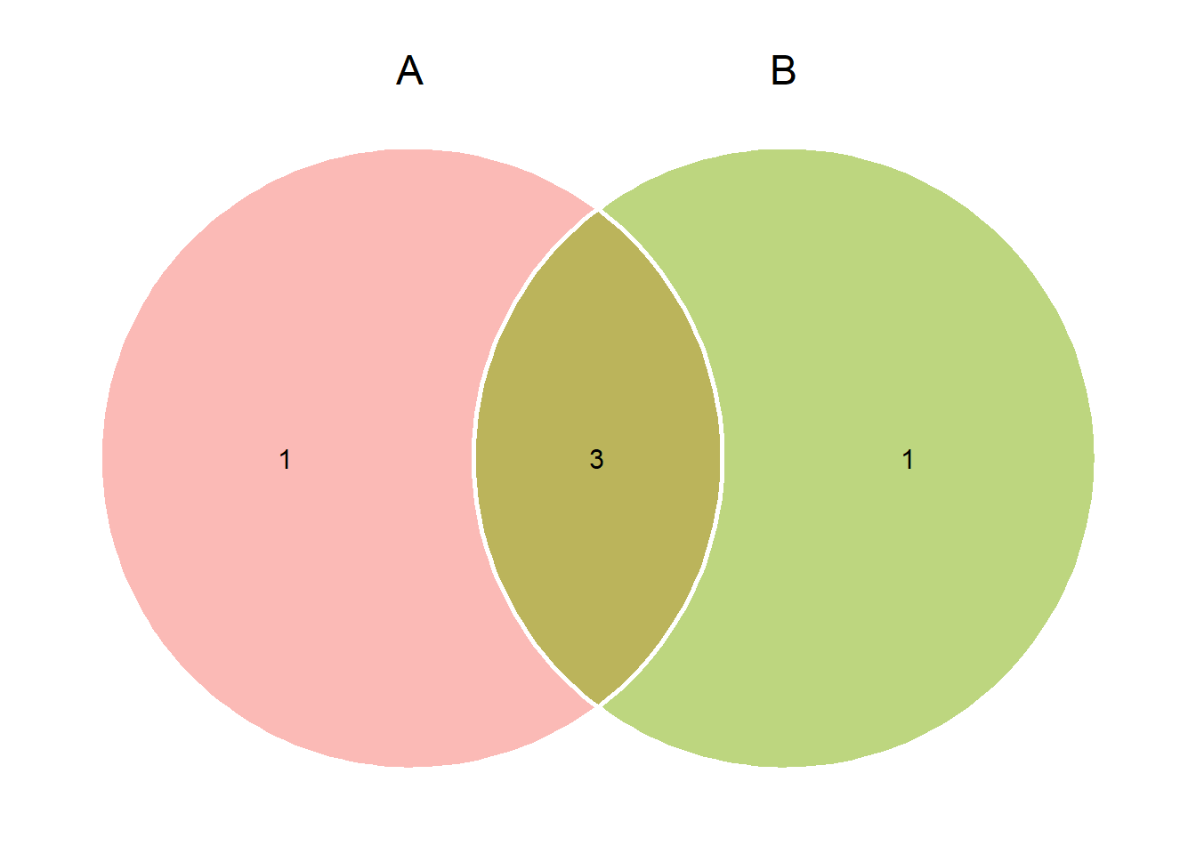
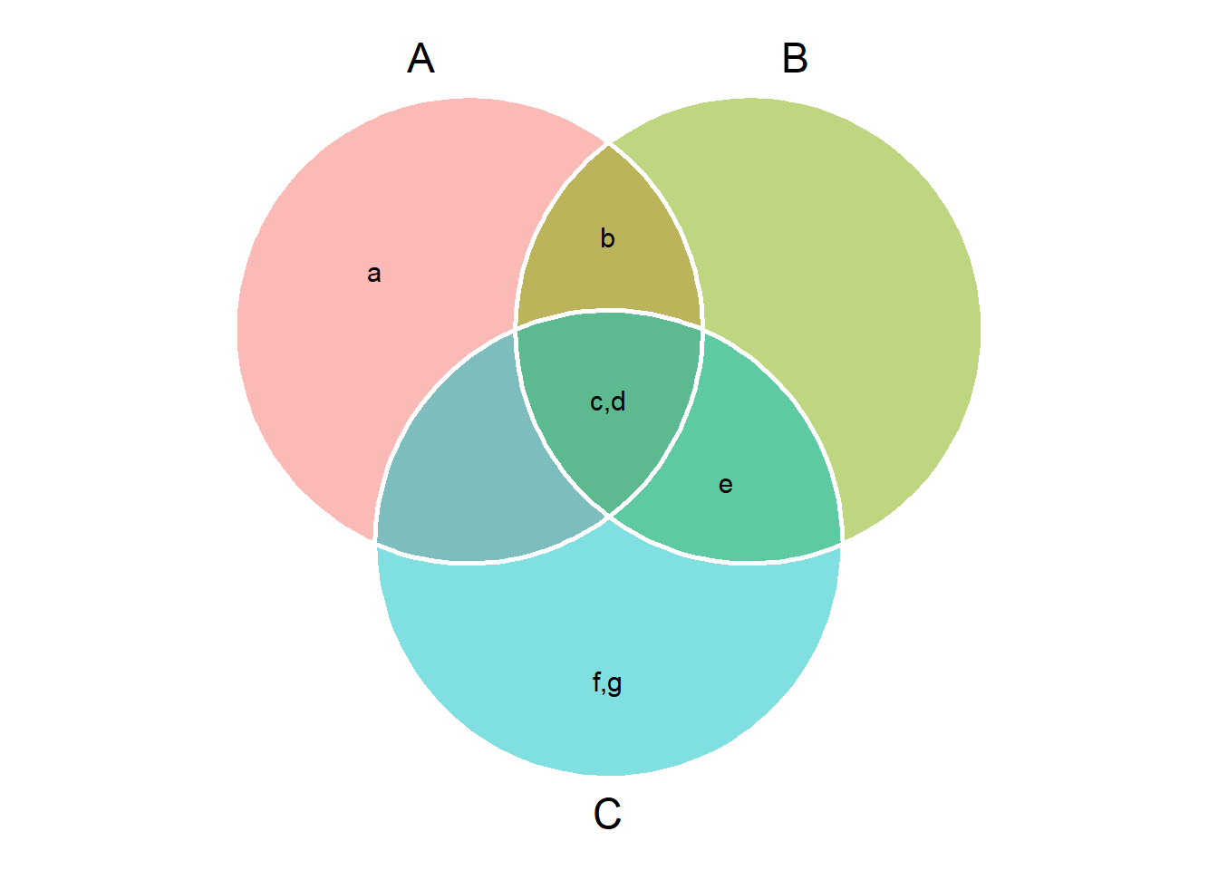
• venn_plot() to compute Venn plots. We can use venn_plot() to compute Venn diagrams with two, three or four sets.

# Two sets
venn_plot(A, B)

# Thre sets
# Show the elements
venn_plot(A, B, C, show_elements = TRUE)

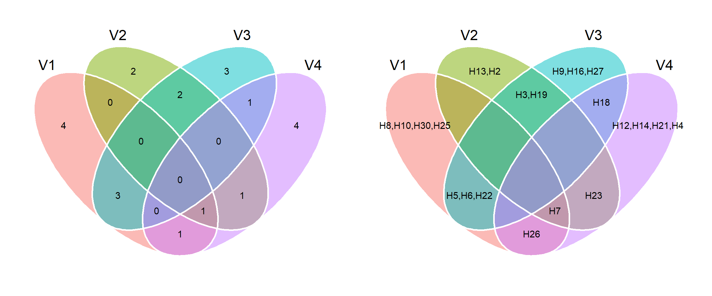
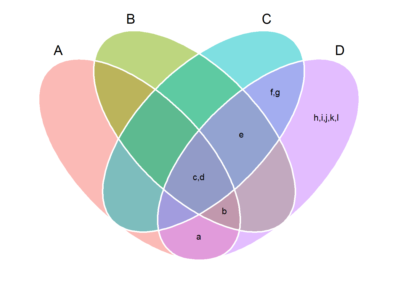
# Four sets
# Show the elements
venn_plot(set_lits, show_elements = TRUE)

A bit more sophisticated example

In the following example, we simulate genotype-environment data with data on four traits analyzed in 30 genotypes growing in 10 environments. We compute the winner genotype within each environment with ge_winner(). Our aim is to define the intersect genotype for the four traits, i.e., the genotype that won in some environment across all the four traits.

df_sets <-
  ge_simula(ngen = 30,
            nenv = 10,
            nrep = 4,
            ge_eff = 100,
            nvars = 4,
            seed = 1:4) # to ensure reproducibility
# Warning: 'gen_eff = 20' recycled for all the 4 traits.
# Warning: 'env_eff = 15' recycled for all the 4 traits.
# Warning: 'rep_eff = 5' recycled for all the 4 traits.
# Warning: 'ge_eff = 100' recycled for all the 4 traits.
# Warning: 'res_eff = 5' recycled for all the 4 traits.
# Warning: 'intercept = 100' recycled for all the 4 traits.
ge_win <- ge_winners(df_sets, ENV, GEN)
winners <- lapply(ge_win[,2:5], function(x){x})
p1 <- venn_plot(winners)
p2 <- venn_plot(winners, show_elements = TRUE)
p1 + p2