metan v1.6.0 on CRAN
I’m so excited to announce that the latest version of the R package
metan is now on
CRAN. This is a minor release (v1.6.0) that includes new features and some minor improvements.
New functions
Smith_Hazel()andprint.sh()andplot.sh()for computing the Smith and Hazel selection index.
The Smith-Hazel index is computed with the function Smith_Hazel(). Users can compute the index either by declaring known genetic and phenotypic variance-covariance matrices or by using as inpute data, a model fitted with the function gamem(). In this case, the variance-covariance are extracted internally. The economic weights in the argument weights are set by default to 1 for all traits.
library(metan)
# Registered S3 method overwritten by 'GGally':
#   method from
#   +.gg   ggplot2
# []=====================================================[]
# [] Multi-Environment Trial Analysis (metan) v1.6.0     []
# [] Author: Tiago Olivoto                               []
# [] Type citation('metan') to know how to cite metan    []
# [] Type vignette('metan_start') for a short tutorial   []
# [] Visit http://bit.ly/2TIq6JE for a complete tutorial []
# []=====================================================[]
mod <- gamem(data_g, GEN, REP, starts_with("N"))
# Method: REML/BLUP
# Random effects: GEN
# Fixed effects: REP
# Denominador DF: Satterthwaite's method
# ---------------------------------------------------------------------------
# P-values for Likelihood Ratio Test of the analyzed traits
# ---------------------------------------------------------------------------
#     model     NR   NKR     NKE
#  Complete     NA    NA      NA
#  Genotype 0.0056 0.216 0.00952
# ---------------------------------------------------------------------------
# Variables with nonsignificant Genotype effect
# NKR
# ---------------------------------------------------------------------------
smith <- Smith_Hazel(mod)
print(smith)
#
# -----------------------------------------------------------------------------------
# Index coefficients
# -----------------------------------------------------------------------------------
# # A tibble: 3 x 3
#   VAR         b gen_weights
#   <chr>   <dbl>       <dbl>
# 1 NR    -11.84            1
# 2 NKR    -9.435           1
# 3 NKE     1.184           1
#
# -----------------------------------------------------------------------------------
# Genetic worth
# -----------------------------------------------------------------------------------
#    GEN        V1
# 1  H13 142.80619
# 2  H12 120.77661
# 3   H5 115.19274
# 4  H10  89.29844
# 5   H4  88.90470
# 6   H2  86.49310
# 7  H11  84.25171
# 8   H7  62.30464
# 9   H1  51.99961
# 10  H3  51.26071
# 11  H6  51.16514
# 12  H9  50.52352
# 13  H8  48.31407
#
# -----------------------------------------------------------------------------------
# Selection gain
# -----------------------------------------------------------------------------------
# # A tibble: 3 x 8
#   VAR       Xo     Xs      SD  SDperc     h2       SG SGperc
#   <chr>  <dbl>  <dbl>   <dbl>   <dbl>  <dbl>    <dbl>  <dbl>
# 1 NR     15.78  16.97  1.189   7.532  0.7359  0.8749  5.543
# 2 NKR    30.40  30.60  0.1960  0.6448 0.4523  0.08866 0.2916
# 3 NKE   467.9  524.9  56.98   12.18   0.7126 40.61    8.678
#
# -----------------------------------------------------------------------------------
# Phenotypic variance-covariance matrix
# -----------------------------------------------------------------------------------
#        NR   NKR  NKE
# NR   1.60  0.13   49
# NKR  0.13  4.75   70
# NKE 48.84 70.12 2782
#
# -----------------------------------------------------------------------------------
# Genotypic variance-covariance matrix
# -----------------------------------------------------------------------------------
#        NR   NKR  NKE
# NR   1.18 -0.18   37
# NKR -0.18  2.15   35
# NKE 36.60 34.72 1982
Minor improvements
get_model_data()now extracts the genotypic and phenotypic variance-covariance matrix from objects of classgamemandwaasb.
get_model_data(mod, "gcov")
# Class of the model: gamem
# Variable extracted: gcov
#            NKE        NKR         NR
# NKE 1982.32081 34.7246852 36.5976336
# NKR   34.72469  2.1466667 -0.1839316
# NR    36.59763 -0.1839316  1.1808547
get_model_data(mod, "pcov")
# Class of the model: gamem
# Variable extracted: pcov
#             NR        NKR        NKE
# NR   1.6045584  0.1303704   48.83903
# NKR  0.1303704  4.7459259   70.11889
# NKE 48.8390313 70.1188889 2781.91453
fai_blup()now returns the total genetic gain and the list with the ideotypes’ construction.
fai <- fai_blup(mod)
#
# -----------------------------------------------------------------------------------
# Principal Component Analysis
# -----------------------------------------------------------------------------------
#     eigen.values cumulative.var
# PC1   1.97579911       65.85997
# PC2   0.95352008       97.64397
# PC3   0.07068081      100.00000
#
# -----------------------------------------------------------------------------------
# Factor Analysis
# -----------------------------------------------------------------------------------
#            FA1 comunalits
# NR  -0.7669378  0.5881937
# NKR -0.6510612  0.4238807
# NKE -0.9816949  0.9637248
#
# -----------------------------------------------------------------------------------
# Comunalit Mean: 0.6585997
# Selection differential
# -----------------------------------------------------------------------------------
# # A tibble: 3 x 9
#   VAR   Factor    Xo    Xs     SD SDperc    h2     SG SGperc
#   <chr>  <dbl> <dbl> <dbl>  <dbl>  <dbl> <dbl>  <dbl>  <dbl>
# 1 NR         1  15.8  17.4  1.63   10.3  0.736  1.20    7.60
# 2 NKR        1  30.4  31.2  0.814   2.68 0.452  0.368   1.21
# 3 NKE        1 468.  532.  64.0    13.7  0.713 45.6     9.74
#
# -----------------------------------------------------------------------------------
# Selected genotypes
# H13 H5
# -----------------------------------------------------------------------------------
mgidi()now computes the genetic gain when a mixed-model is used as input data.
mgidi_index <- mgidi(mod)
#
# -------------------------------------------------------------------------------
# Principal Component Analysis
# -------------------------------------------------------------------------------
# # A tibble: 3 x 4
#   PC    Eigenvalues `Variance (%)` `Cum. variance (%)`
#   <chr>       <dbl>          <dbl>               <dbl>
# 1 PC1        1.98            65.9                 65.9
# 2 PC2        0.954           31.8                 97.6
# 3 PC3        0.0707           2.36               100
# -------------------------------------------------------------------------------
# Factor Analysis - factorial loadings after rotation-
# -------------------------------------------------------------------------------
# # A tibble: 3 x 4
#   VAR      FA1 Communality Uniquenesses
#   <chr>  <dbl>       <dbl>        <dbl>
# 1 NR    -0.767       0.588       0.412
# 2 NKR   -0.651       0.424       0.576
# 3 NKE   -0.982       0.964       0.0363
# -------------------------------------------------------------------------------
# Comunalit Mean: 0.6585997
# -------------------------------------------------------------------------------
# Selection differential
# -------------------------------------------------------------------------------
# # A tibble: 3 x 10
#   VAR   Factor    Xo    Xs     SD SDperc    h2     SG SGperc sense
#   <chr> <chr>  <dbl> <dbl>  <dbl>  <dbl> <dbl>  <dbl>  <dbl> <chr>
# 1 NR    FA 1    15.8  17.4  1.63   10.3  0.736  1.20    7.60 increase
# 2 NKR   FA 1    30.4  31.2  0.814   2.68 0.452  0.368   1.21 increase
# 3 NKE   FA 1   468.  532.  64.0    13.7  0.713 45.6     9.74 increase
# ------------------------------------------------------------------------------
# Selected genotypes
# -------------------------------------------------------------------------------
# H13 H5
# -------------------------------------------------------------------------------
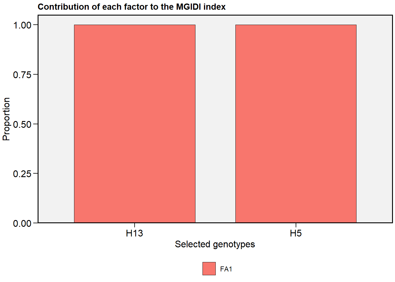
- The S3 method
plot()for objects of classmgidihas a new argumenttype = "contribution"to plot the contribution of each factor in the MGIDI index.
plot(mgidi_index, type = "contribution")
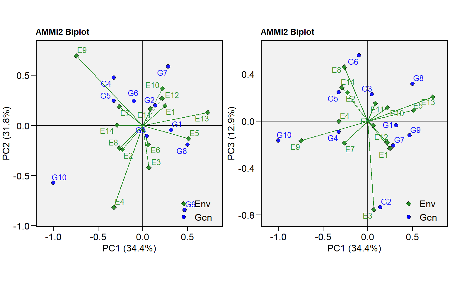
plot_scores()now can produce a biplot showing other axes besides PC1 and PC2. To change the default IPCA in each axis use the new argumentsfirstandsecond.
ammi <- performs_ammi(data_ge, ENV, GEN, REP, GY)
# variable GY
# ---------------------------------------------------------------------------
# AMMI analysis table
# ---------------------------------------------------------------------------
#     Source  Df  Sum Sq Mean Sq F value   Pr(>F) Proportion Accumulated
#        ENV  13 279.574 21.5057   62.33 0.00e+00          .           .
#   REP(ENV)  28   9.662  0.3451    3.57 3.59e-08          .           .
#        GEN   9  12.995  1.4439   14.93 2.19e-19          .           .
#    GEN:ENV 117  31.220  0.2668    2.76 1.01e-11          .           .
#        PC1  21  10.749  0.5119    5.29 0.00e+00       34.4        34.4
#        PC2  19   9.924  0.5223    5.40 0.00e+00       31.8        66.2
#        PC3  17   4.039  0.2376    2.46 1.40e-03       12.9        79.2
#        PC4  15   3.074  0.2049    2.12 9.60e-03        9.8          89
#        PC5  13   1.446  0.1113    1.15 3.18e-01        4.6        93.6
#        PC6  11   0.932  0.0848    0.88 5.61e-01          3        96.6
#        PC7   9   0.567  0.0630    0.65 7.53e-01        1.8        98.4
#        PC8   7   0.362  0.0518    0.54 8.04e-01        1.2        99.6
#        PC9   5   0.126  0.0252    0.26 9.34e-01        0.4         100
#  Residuals 252  24.367  0.0967      NA       NA          .           .
#      Total 536 389.036  0.7258      NA       NA       <NA>        <NA>
# ---------------------------------------------------------------------------
#
# All variables with significant (p < 0.05) genotype-vs-environment interaction
# Done!
p1 <- plot_scores(ammi, type = 2)
p2 <- plot_scores(ammi, type = 2, second = "PC3")
arrange_ggplot(p1, p2)
Find out more about metan at https://tiagoolivoto.github.io/metan/