metan 1.17.0 is now available!
 Image by jplenio from Pixabay
After exactly seven months since the last stable release, I’m chuffed to announce that metan 1.17.0 in now on
CRAN. metan was first released on CRAN on 2020/01/14 and since there, 16 stable versions have been released regularly. I’m happy with the package cause today it does much more than it was designed to do. So, from now on, stable versions gonna be launched within a wider time interval, mainly cause I’m now focused on improving the
pliman package. Critical bug fixes and minor improvements, however, can be quickly obtained from the
dev version.
This new version includes new features and minor improvements, that I’ll dissect below.
Instalation
# The latest stable version is installed with
install.packages("metan")

# Or the development version from GitHub:
# install.packages("devtools")
devtools::install_github("TiagoOlivoto/metan")
New features
- This new version includes a new function
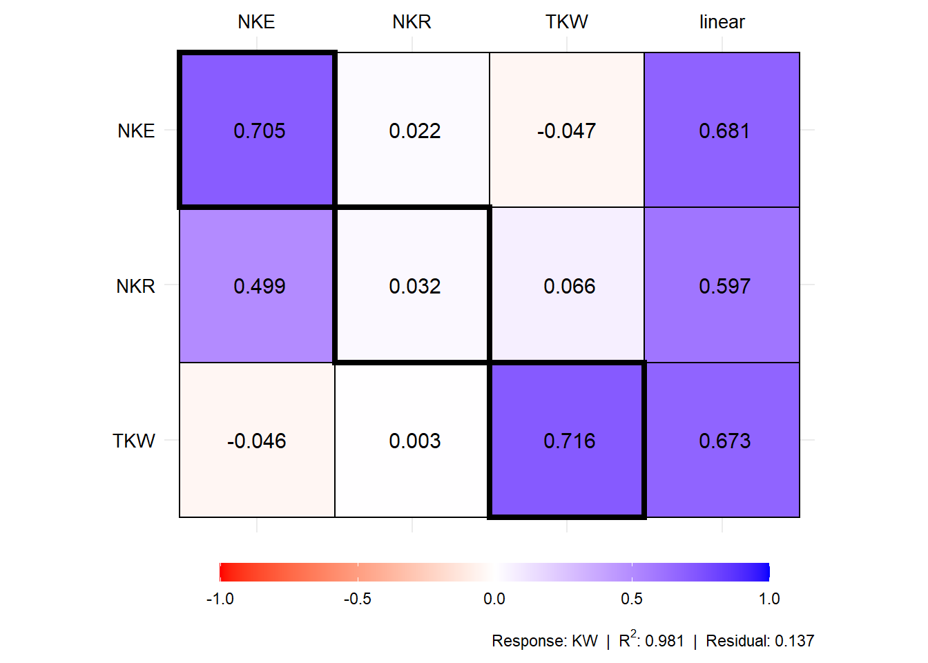
path_coeff_seq()to implement a sequential (two chains) path analysis (see more details in this blogpost).
library(metan)
# Registered S3 method overwritten by 'GGally':
#   method from
#   +.gg   ggplot2
# |=========================================================|
# | Multi-Environment Trial Analysis (metan) v1.17.0        |
# | Author: Tiago Olivoto                                   |
# | Type 'citation('metan')' to know how to cite metan      |
# | Type 'vignette('metan_start')' for a short tutorial     |
# | Visit 'https://bit.ly/pkgmetan' for a complete tutorial |
# |=========================================================|

mod1 <-
  path_coeff_seq(data_ge2,
                 resp = KW,
                 chain_1 = c(TKW, NKE, NKR),
                 chain_2 = c(PH, EH, EL, ED, CL, CD))
# ========================================================
# Collinearity diagnosis of first chain predictors
# ========================================================
# Weak multicollinearity.
# Condition Number: 6.214
# You will probably have path coefficients close to being unbiased.
# ========================================================
# Collinearity diagnosis of second chain predictors
# ========================================================
# Weak multicollinearity.
# Condition Number: 66.559
# You will probably have path coefficients close to being unbiased.
mod1$fc_sc_coef
#       trait     effects         TKW          NKE         NKR
# 1        PH      direct  0.37945659 -0.004890662 -0.25616717
# 2        PH indirect_EH -0.05289378  0.017147221  0.39976851
# 3        PH indirect_EL  0.03394241  0.115204549  0.07929626
# 4        PH indirect_ED  0.03524760  0.518887963  0.18215663
# 5        PH indirect_CL  0.13816764 -0.189545091 -0.18742353
# 6        PH indirect_CD  0.03461798  0.001576069  0.13541882
# 7        PH      linear  0.56853845  0.458380049  0.35304952
# 8        EH indirect_PH  0.35358835 -0.004557257 -0.23870380
# 9        EH      direct -0.05676344  0.018401697  0.42901525
# 10       EH indirect_EL  0.03237631  0.109889000  0.07563752
# 11       EH indirect_ED  0.03359219  0.494518292  0.17360161
# 12       EH indirect_CL  0.16877378 -0.231532069 -0.22894055
# 13       EH indirect_CD  0.03078957  0.001401771  0.12044283
# 14       EH      linear  0.56235676  0.388121434  0.33105286
# 15       EL indirect_PH  0.14426788 -0.001859410 -0.09739374
# 16       EL indirect_EH -0.02058548  0.006673444  0.15558398
# 17       EL      direct  0.08927609  0.303013563  0.20856678
# 18       EL indirect_ED  0.02052796  0.302196714  0.10608674
# 19       EL indirect_CL  0.10852635 -0.148881721 -0.14721530
# 20       EL indirect_CD  0.10008828  0.004556765  0.39152587
# 21       EL      linear  0.44210108  0.465699355  0.61715434
# 22       ED indirect_PH  0.25094027 -0.003234267 -0.16940715
# 23       ED indirect_EH -0.03577550  0.011597781  0.27038946
# 24       ED indirect_EL  0.03438425  0.116704196  0.08032848
# 25       ED      direct  0.05329928  0.784630768  0.27544616
# 26       ED indirect_CL  0.29636296 -0.406565110 -0.40201446
# 27       ED indirect_CD  0.04277571  0.001947469  0.16733026
# 28       ED      linear  0.64198696  0.505080838  0.22207274
# 29       CL indirect_PH  0.12338593 -0.001590271 -0.08329655
# 30       CL indirect_EH -0.02254607  0.007309035  0.17040208
# 31       CL indirect_EL  0.02280172  0.077391712  0.05326936
# 32       CL indirect_ED  0.03717427  0.547250848  0.19211348
# 33       CL      direct  0.42491573 -0.582920055 -0.57639548
# 34       CL indirect_CD  0.03296855  0.001500974  0.12896657
# 35       CL      linear  0.61870013  0.048942243 -0.11494054
# 36       CD indirect_PH  0.11967718 -0.001542470 -0.08079281
# 37       CD indirect_EH -0.01592282  0.005161893  0.12034384
# 38       CD indirect_EL  0.08140777  0.276307542  0.19018480
# 39       CD indirect_ED  0.02077141  0.305780671  0.10734490
# 40       CD indirect_CL  0.12762923 -0.175087987 -0.17312824
# 41       CD      direct  0.10976213  0.004997191  0.42936812
# 42       CD      linear  0.44332490  0.415616840  0.59332061
# 43       R2          R2  0.56905656  0.515863000  0.56247816
# 44 Residual    Residual  0.65646283  0.695799540  0.66145433

# Coefficients for the primary traits and response
plot(mod1$resp_fc)
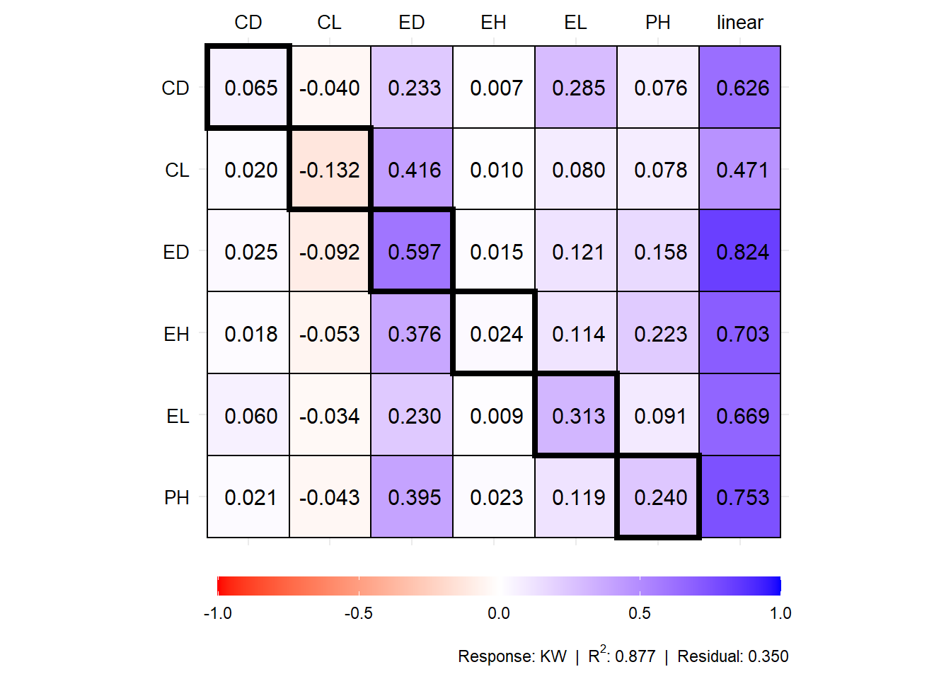
# Coefficients for the secondary traits and response
plot(mod1$resp_sc)
- New functions
ci_mean_z()andci_mean_t()to compute z- and t-confidence intervals, respectively. Let’s see how the confidence interval changes depending on the different sample sizes.
df <- data.frame(data = rnorm(n = 20, mean = 30, sd = 10))
m <- mean(df$data)
dp <- sd(df$data)
n <- 20

# t-interval (95%)
qt(0.975, 19) * dp / sqrt(n)
# [1] 4.610762
ci_mean_t(df)
#       data
# 1 4.610762

# z-interval (95%)
qnorm(0.975) * dp / sqrt(n)
# [1] 4.317642
ci_mean_z(df)
#       data
# 1 4.317642


# now in a data frame with several traits
ci_mean_t(data_ge2)
# # A tibble: 1 × 15
#       PH     EH      EP    EL    ED    CL    CD    CW    KW    NR   NKR    CDED
#    <dbl>  <dbl>   <dbl> <dbl> <dbl> <dbl> <dbl> <dbl> <dbl> <dbl> <dbl>   <dbl>
# 1 0.0528 0.0450 0.00891 0.199 0.437 0.365 0.185 0.990  5.18 0.259 0.548 0.00529
# # … with 3 more variables: PERK <dbl>, TKW <dbl>, NKE <dbl>
- New function
prop_na()to measure the proportion of NAs in each column.
# force 20% of NA in GY
dfna <- data_ge
dfna[sample(1:nrow(dfna), 84), 4] <- NA
prop_na(dfna)
#   variable prop
# 1      ENV  0.0
# 2      GEN  0.0
# 3      REP  0.0
# 4       GY  0.2
# 5       HM  0.0
- New functions
remove_cols_all_na()andremove_rows_all_na()to remove columns and rows that have all values as NAs.
dfna$HM <- NA

# see the difference
remove_cols_na(dfna)
# Warning: Column(s) GY, HM with NA values deleted.
# # A tibble: 420 × 3
#    ENV   GEN   REP
#    <fct> <fct> <fct>
#  1 E1    G1    1
#  2 E1    G1    2
#  3 E1    G1    3
#  4 E1    G2    1
#  5 E1    G2    2
#  6 E1    G2    3
#  7 E1    G3    1
#  8 E1    G3    2
#  9 E1    G3    3
# 10 E1    G4    1
# # … with 410 more rows
remove_cols_all_na(dfna)
# Warning: Column(s) HM with all NA values deleted.
# # A tibble: 420 × 4
#    ENV   GEN   REP      GY
#    <fct> <fct> <fct> <dbl>
#  1 E1    G1    1      2.17
#  2 E1    G1    2      2.50
#  3 E1    G1    3     NA
#  4 E1    G2    1      3.21
#  5 E1    G2    2      2.93
#  6 E1    G2    3      2.56
#  7 E1    G3    1      2.77
#  8 E1    G3    2      3.62
#  9 E1    G3    3      2.28
# 10 E1    G4    1     NA
# # … with 410 more rows
-
New functions
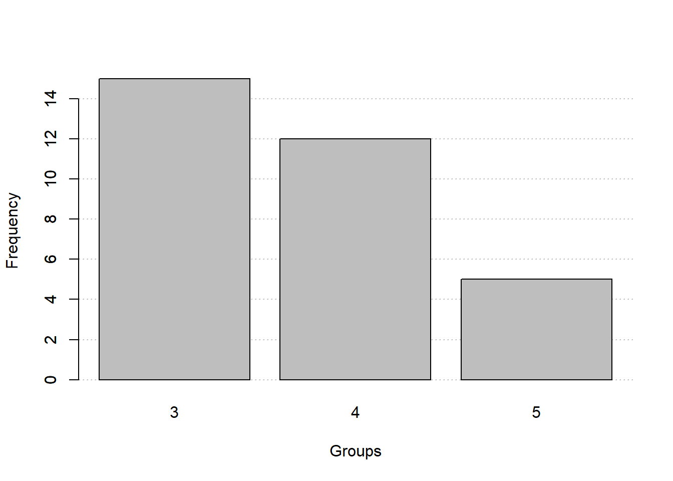
freq_table()andfreq_hist()to create frequency tables and histograms, respectively.- Qualitative or continuous-discrete variables
fq_quali <-
  mtcars |>
  as_integer(gear) |>
  freq_table(gear)
fq_quali$freqs
#    gear abs_freq abs_freq_ac rel_freq rel_freq_ac
# 1     3       15          15    0.469       0.469
# 2     4       12          27    0.375       0.844
# 3     5        5          32    0.156       1.000
# 4 Total       32          32    1.000       1.000

# histogram
freq_hist(fq_quali)
- Continuous variables
# default number of classes [sqrt(n)]
fq_quanti <-
mtcars |>
freq_table(wt)
# Warning: An empty class is not advised. Try to reduce the number of classes with
# the `k` argument
fq_quanti$freqs
# class abs_freq abs_freq_ac rel_freq rel_freq_ac
# 1 1.122 |--- 1.904 3 3 0.094 0.094
# 2 1.904 |--- 2.686 6 9 0.188 0.281
# 3 2.686 |--- 3.468 12 21 0.375 0.656
# 4 3.468 |--- 4.25 8 29 0.250 0.906
# 5 4.25 |--- 5.032 0 29 0.000 0.906
# 6 5.032 |---| 5.814 3 32 0.094 1.000
# 7 Total 32 32 1.000 1.000
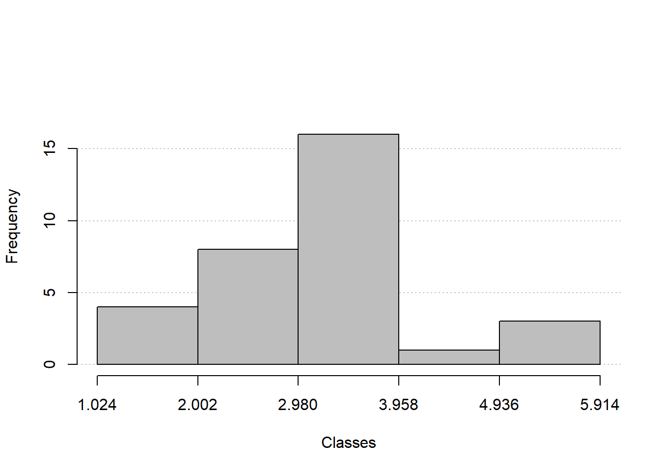
# change the number of classes
fq_quanti2 <-
mtcars |>
freq_table(wt, k = 5)
fq_quanti2$freqs
# class abs_freq abs_freq_ac rel_freq rel_freq_ac
# 1 1.024 |--- 2.002 4 4 0.125 0.125
# 2 2.002 |--- 2.98 8 12 0.250 0.375
# 3 2.98 |--- 3.958 16 28 0.500 0.875
# 4 3.958 |--- 4.936 1 29 0.031 0.906
# 5 4.936 |---| 5.914 3 32 0.094 1.000
# 6 Total 32 32 1.000 1.000
freq_hist(fq_quanti2)
Minor improvements
- Improve the control over highlighted individuals in
plot_scores(), such as shape, alpha, color, and size. - Fix bug with
x.labandy.labfromplot_scores(). Now it accepts an object fromexpression()
# WAASB model
model <- waasb(data_ge,
env = ENV,
gen = GEN,
rep = REP,
resp = GY)
# Evaluating trait GY |============================================| 100% 00:00:01
# Method: REML/BLUP
# Random effects: GEN, GEN:ENV
# Fixed effects: ENV, REP(ENV)
# Denominador DF: Satterthwaite's method
# ---------------------------------------------------------------------------
# P-values for Likelihood Ratio Test of the analyzed traits
# ---------------------------------------------------------------------------
# model GY
# COMPLETE NA
# GEN 1.11e-05
# GEN:ENV 2.15e-11
# ---------------------------------------------------------------------------
# All variables with significant (p < 0.05) genotype-vs-environment interaction
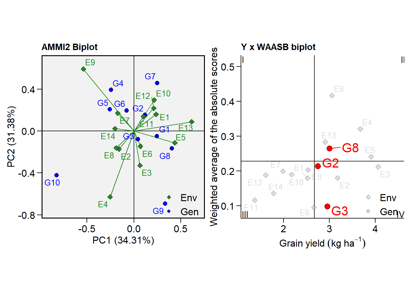
# PC1 x PC1
p1 <- plot_scores(model, type = 2)
# WAASB x GY
p2 <- plot_scores(model,
type = 3,
x.lab = expression(Grain~yield~(kg~ha^{-1})),
highlight = c("G2", "G3", "G8"), #highlight genotypes
col.alpha.env = 0.5, # alpha for environments
col.alpha.gen = 0, # remove the other genotypes
col.env = "gray", # color for environment point
col.segm.env = "gray", # color for environment segment
plot_theme = theme_metan_minimal()) # theme
arrange_ggplot(p1, p2)
get_model_data()now includes new options coefs, and anova for objects computed withge_reg().
reg <- ge_reg(data_ge2,
             env = ENV,
             gen = GEN,
             rep = REP,
             resp = PH)
# Evaluating trait PH |============================================| 100% 00:00:00
get_model_data(reg, what = "coefs")
# Class of the model: ge_reg
# Variable extracted: coefs
# # A tibble: 13 × 11
#    TRAIT GEN      b0    b1 `t(b1=1)`[,1] pval_t[,1]   s2di `F(s2di=0)`    pval_f
#    <chr> <chr> <dbl> <dbl>         <dbl>      <dbl>  <dbl>       <dbl>     <dbl>
#  1 PH    H1     2.62 0.806       -0.997    0.321    0.0710       10.5    7.56e-5
#  2 PH    H10    2.31 1.22         1.12     0.265    0.0318        5.25   6.85e-3
#  3 PH    H11    2.39 1.08         0.411    0.682    0.0278        4.71   1.12e-2
#  4 PH    H12    2.44 0.465       -2.75     0.00711  0.0676       10.0    1.10e-4
#  5 PH    H13    2.54 0.306       -3.57     0.000558 0.0609        9.15   2.31e-4
#  6 PH    H2     2.60 0.963       -0.188    0.851    0.0815       11.9    2.41e-5
#  7 PH    H3     2.59 1.35         1.83     0.0711   0.0898       13.0    9.95e-6
#  8 PH    H4     2.58 1.27         1.38     0.171    0.0515        7.89   6.71e-4
#  9 PH    H5     2.57 1.17         0.887    0.378    0.0159        3.13   4.84e-2
# 10 PH    H6     2.56 0.936       -0.330    0.742    0.0481        7.44   9.94e-4
# 11 PH    H7     2.40 0.992       -0.0393   0.969    0.0328        5.38   6.09e-3
# 12 PH    H8     2.33 1.01         0.0720   0.943    0.0767       11.3    4.03e-5
# 13 PH    H9     2.36 1.42         2.18     0.0317   0.0212        3.84   2.49e-2
# # … with 2 more variables: RMSE <dbl>, R2 <dbl>
get_model_data(reg, what = "anova")
# Class of the model: ge_reg
# Variable extracted: anova
# # A tibble: 20 × 7
#    TRAIT SV                       Df `Sum Sq` `Mean Sq` `F value`    `Pr(>F)`
#    <chr> <chr>                 <dbl>    <dbl>     <dbl>     <dbl>       <dbl>
#  1 PH    "Total"                  51   15.0      0.294     NA     NA
#  2 PH    "GEN"                    12    1.86     0.155      0.870  0.585
#  3 PH    "ENV + (GEN x ENV)"      39   13.1      0.336     NA     NA
#  4 PH    "ENV (linear)"            1    7.72     7.72      NA     NA
#  5 PH    " GEN x ENV (linear)"    12    0.755    0.0629     0.352  0.969
#  6 PH    "Pooled deviation"       26    4.64     0.179     NA     NA
#  7 PH    "H1"                      2    0.471    0.235     10.5    0.0000756
#  8 PH    "H10"                     2    0.236    0.118      5.25   0.00685
#  9 PH    "H11"                     2    0.211    0.106      4.71   0.0112
# 10 PH    "H12"                     2    0.450    0.225     10.0    0.000110
# 11 PH    "H13"                     2    0.410    0.205      9.15   0.000231
# 12 PH    "H2"                      2    0.534    0.267     11.9    0.0000241
# 13 PH    "H3"                      2    0.584    0.292     13.0    0.00000995
# 14 PH    "H4"                      2    0.354    0.177      7.89   0.000671
# 15 PH    "H5"                      2    0.140    0.0701     3.13   0.0484
# 16 PH    "H6"                      2    0.334    0.167      7.44   0.000994
# 17 PH    "H7"                      2    0.241    0.121      5.38   0.00609
# 18 PH    "H8"                      2    0.505    0.253     11.3    0.0000403
# 19 PH    "H9"                      2    0.172    0.0861     3.84   0.0249
# 20 PH    "Pooled error"           96    2.15     0.0224    NA     NA
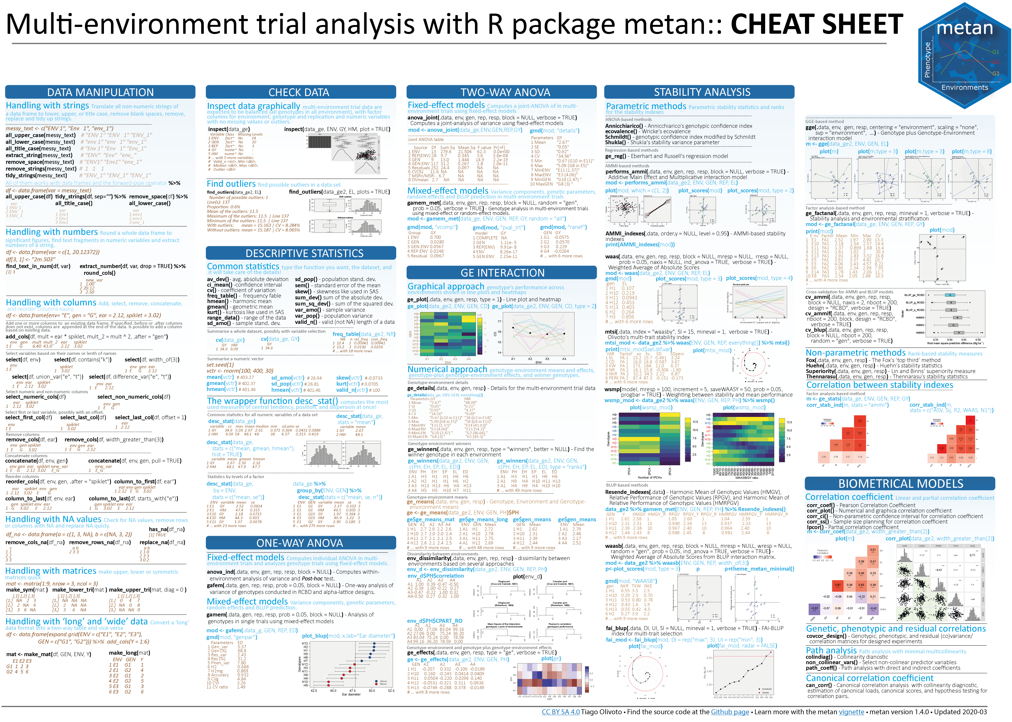
Cheatsheet
Citation
To cite metan in your publications, please, use the official reference paper:
Olivoto, T., and Lúcio, A.D. (2020). metan: an R package for multi-environment trial analysis. Methods Ecol Evol. 11:783-789 doi: 10.1111/2041-210X.13384
A BibTeX entry for LaTeX users is
@Article{Olivoto2020,
author = {Tiago Olivoto and Alessandro Dal'Col L{'{u}}cio},
title = {metan: an R package for multi-environment trial analysis},
journal = {Methods in Ecology and Evolution},
volume = {11},
number = {6},
pages = {783-789},
year = {2020},
doi = {10.1111/2041-210X.13384},
}