Sequential path analysis with {metan} R package
 Image by TanteTati from Pixabay
Studying relationships among crop traits is crucial for the understanding of complex biological systems that occur in plants. Some traits develop earlier in ontogeny and affect other traits that develop later. Therefore, a sequential path analysis should be a better option to study cause-and-effect relationships where one trait affects another trait.
For a long time, it was on my radar to implement an option to perform sequential path analysis in metan. The final push into this topic was given during
Gabrielle Lombardi’s doctoral thesis defense, where I was participating as a member of the examination committee. Gabrielli used metan for most of her analysis and has been questioned why the sequential path analysis was done with other software. Since metan has a function to perform path analysis, I realized that it should be not so laborious to implement a routine for sequential path analysis; and here we are; better late than never!
The function to implement path analysis in {metan} is
path_analysis_seq(). To use this function, the development version of metan must be installed.
Instalation
devtools::install_github("TiagoOlivoto/pliman")
A numerical example.
In this short post, I’ll use the data data_ge2(), a data set for a maize multi-environment trial, as a motivating example. The BLUPs for the genotype-environment interaction will be used in the path analysis in two ways. The first will consider the analysis across environments. In the second, a sequential path analysis will be performed within each environment.
To construct the sequential model, KW (kernel weight per ear) will be used as the dependent trait. The first set of predictors will be TKW, NKE, and NKR. The second set of predictors will be the plant- and ear-related traits PH, EH, EL, ED, CL, and CD.
library(metan)
# Registered S3 method overwritten by 'GGally':
#   method from
#   +.gg   ggplot2
# |=========================================================|
# | Multi-Environment Trial Analysis (metan) v1.16.0        |
# | Author: Tiago Olivoto                                   |
# | Type 'citation('metan')' to know how to cite metan      |
# | Type 'vignette('metan_start')' for a short tutorial     |
# | Visit 'https://bit.ly/pkgmetan' for a complete tutorial |
# |=========================================================|
str(data_ge2)
# tibble [156 x 18] (S3: tbl_df/tbl/data.frame)
#  $ ENV : Factor w/ 4 levels "A1","A2","A3",..: 1 1 1 1 1 1 1 1 1 1 ...
#  $ GEN : Factor w/ 13 levels "H1","H10","H11",..: 1 1 1 2 2 2 3 3 3 4 ...
#  $ REP : Factor w/ 3 levels "1","2","3": 1 2 3 1 2 3 1 2 3 1 ...
#  $ PH  : num [1:156] 2.61 2.87 2.68 2.83 2.79 ...
#  $ EH  : num [1:156] 1.71 1.76 1.58 1.64 1.71 ...
#  $ EP  : num [1:156] 0.658 0.628 0.591 0.581 0.616 ...
#  $ EL  : num [1:156] 16.1 14.2 16 16.7 14.9 ...
#  $ ED  : num [1:156] 52.2 50.3 50.7 54.1 52.7 ...
#  $ CL  : num [1:156] 28.1 27.6 28.4 31.7 32 ...
#  $ CD  : num [1:156] 16.3 14.5 16.4 17.4 15.5 ...
#  $ CW  : num [1:156] 25.1 21.4 24 26.2 20.7 ...
#  $ KW  : num [1:156] 217 184 208 194 176 ...
#  $ NR  : num [1:156] 15.6 16 17.2 15.6 17.6 16.8 16.8 13.6 15.2 14.8 ...
#  $ NKR : num [1:156] 36.6 31.4 31.8 32.8 28 32.8 34.6 34.4 34.8 31.6 ...
#  $ CDED: num [1:156] 0.538 0.551 0.561 0.586 0.607 ...
#  $ PERK: num [1:156] 89.6 89.5 89.7 87.9 89.7 ...
#  $ TKW : num [1:156] 418 361 367 374 347 ...
#  $ NKE : num [1:156] 521 494 565 519 502 ...
blups <-
  gamem_met(data_ge2,
            env = ENV,
            gen = GEN,
            rep = REP,
            resp = everything()) %>%
  gmd(what = "blupge")
# Evaluating trait PH |===                                         | 7% 00:00:00
Evaluating trait EH |======                                      | 13% 00:00:00
Evaluating trait EP |=========                                   | 20% 00:00:01
Evaluating trait EL |============                                | 27% 00:00:01
Evaluating trait ED |===============                             | 33% 00:00:01
Evaluating trait CL |==================                          | 40% 00:00:02
Evaluating trait CD |=====================                       | 47% 00:00:02
Evaluating trait CW |=======================                     | 53% 00:00:02
Evaluating trait KW |==========================                  | 60% 00:00:03
Evaluating trait NR |=============================               | 67% 00:00:03
Evaluating trait NKR |================================           | 73% 00:00:03
Evaluating trait CDED |==================================        | 80% 00:00:04
Evaluating trait PERK |====================================      | 87% 00:00:04
Evaluating trait TKW |========================================   | 93% 00:00:04
Evaluating trait NKE |===========================================| 100% 00:00:05
# Method: REML/BLUP
# Random effects: GEN, GEN:ENV
# Fixed effects: ENV, REP(ENV)
# Denominador DF: Satterthwaite's method
# ---------------------------------------------------------------------------
# P-values for Likelihood Ratio Test of the analyzed traits
# ---------------------------------------------------------------------------
#     model       PH       EH       EP      EL       ED       CL       CD
#  COMPLETE       NA       NA       NA      NA       NA       NA       NA
#       GEN 9.39e-01 1.00e+00 1.00e+00 1.00000 2.99e-01 1.00e+00 0.757438
#   GEN:ENV 1.09e-13 8.12e-12 1.97e-05 0.00103 1.69e-08 9.62e-17 0.000429
#        CW       KW       NR     NKR     CDED     PERK      TKW     NKE
#        NA       NA       NA      NA       NA       NA       NA      NA
#  1.00e+00 6.21e-01 1.00e+00 0.78738 1.00e+00 1.00e+00 1.00e+00 1.00000
#  4.93e-14 4.92e-07 4.88e-05 0.00404 7.03e-13 3.86e-17 4.21e-10 0.00101
# ---------------------------------------------------------------------------
# All variables with significant (p < 0.05) genotype-vs-environment interaction
# Class of the model: waasb
# Variable extracted: blupge
Across environments
mod1 <-
  path_coeff_seq(blups,
                 resp = KW,
                 chain_1 = c(TKW, NKE, NKR),
                 chain_2 = c(PH, EH, EL, ED, CL, CD))
# ========================================================
# Collinearity diagnosis of first chain predictors
# ========================================================
# Weak multicollinearity.
# Condition Number: 11.92
# You will probably have path coefficients close to being unbiased.
# ========================================================
# Collinearity diagnosis of second chain predictors
# ========================================================
# Moderate multicollinearity!
# Condition Number: 179.285
# Please, cautiosely evaluate the VIF and matrix determinant.

# Coefficients for the primary traits and response
plot(mod1$resp_fc)

# Coefficients for the secondary traits and response
plot(mod1$resp_sc)
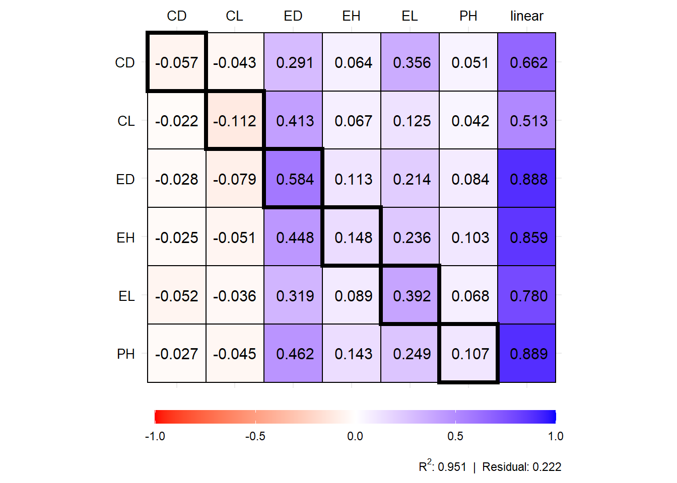
# contribution to the total effects through primary traits
gmd(mod1) %>% round_cols(digits = 3)
# Class of the model: path_coeff_seq
# Variable extracted: resp_sc2
#    trait      effect   TKW    NKE    NKR residual  total
# 1     PH      direct 0.165  0.030 -0.008    0.081  0.107
# 2     PH indirect_EH 0.054  0.035  0.013   -0.041  0.143
# 3     PH indirect_EL 0.037  0.201  0.007   -0.004  0.249
# 4     PH indirect_ED 0.010  0.399  0.005   -0.047  0.462
# 5     PH indirect_CL 0.117 -0.141 -0.005    0.016 -0.045
# 6     PH indirect_CD 0.027 -0.059  0.001   -0.002 -0.027
# 7     PH       total 0.411  0.467  0.014    0.002  0.889
# 8     EH      direct 0.056  0.037  0.013   -0.042  0.148
# 9     EH indirect_PH 0.160  0.029 -0.008    0.078  0.103
# 10    EH indirect_EL 0.035  0.190  0.006   -0.004  0.236
# 11    EH indirect_ED 0.010  0.388  0.005   -0.046  0.448
# 12    EH indirect_CL 0.134 -0.161 -0.006    0.018 -0.051
# 13    EH indirect_CD 0.025 -0.053  0.001   -0.002 -0.025
# 14    EH       total 0.419  0.429  0.013    0.002  0.859
# 15    EL      direct 0.059  0.316  0.011   -0.006  0.392
# 16    EL indirect_PH 0.105  0.019 -0.005    0.051  0.068
# 17    EL indirect_EH 0.034  0.022  0.008   -0.025  0.089
# 18    EL indirect_ED 0.007  0.276  0.004   -0.032  0.319
# 19    EL indirect_CL 0.094 -0.113 -0.004    0.012 -0.036
# 20    EL indirect_CD 0.052 -0.111  0.003   -0.005 -0.052
# 21    EL       total 0.350  0.409  0.016   -0.005  0.780
# 22    ED      direct 0.013  0.506  0.006   -0.059  0.584
# 23    ED indirect_PH 0.131  0.024 -0.006    0.064  0.084
# 24    ED indirect_EH 0.043  0.028  0.010   -0.032  0.113
# 25    ED indirect_EL 0.032  0.172  0.006   -0.004  0.214
# 26    ED indirect_CL 0.208 -0.251 -0.009    0.028 -0.079
# 27    ED indirect_CD 0.028 -0.061  0.001   -0.003 -0.028
# 28    ED       total 0.455  0.418  0.009   -0.006  0.888
# 29    CL      direct 0.294 -0.355 -0.012    0.039 -0.112
# 30    CL indirect_PH 0.066  0.012 -0.003    0.032  0.042
# 31    CL indirect_EH 0.025  0.017  0.006   -0.019  0.067
# 32    CL indirect_EL 0.019  0.101  0.003   -0.002  0.125
# 33    CL indirect_ED 0.009  0.357  0.005   -0.042  0.413
# 34    CL indirect_CD 0.022 -0.046  0.001   -0.002 -0.022
# 35    CL       total 0.435  0.085  0.000    0.006  0.513
# 36    CD      direct 0.057 -0.122  0.003   -0.005 -0.057
# 37    CD indirect_PH 0.079  0.014 -0.004    0.039  0.051
# 38    CD indirect_EH 0.024  0.016  0.006   -0.018  0.064
# 39    CD indirect_EL 0.053  0.287  0.010   -0.006  0.356
# 40    CD indirect_ED 0.006  0.251  0.003   -0.030  0.291
# 41    CD indirect_CL 0.112 -0.135 -0.005    0.015 -0.043
# 42    CD       total 0.332  0.312  0.013   -0.005  0.662
within environments
To perform the path analysis for each level of a factor (or combination of factors), we can use the argument by. In this case, I’ll compute the model above for each environment in data_ge2.
mod2 <-
  path_coeff_seq(blups,
                 resp = KW,
                 chain_1 = c(TKW, NKE, NKR),
                 chain_2 = c(PH, EH, EL, ED, CL, CD),
                 by = ENV,
                 verbose = FALSE)


# contribution to the total effects through primary traits
gmd(mod2) %>% round_cols(digits = 3)
# Class of the model: group_path_seq, tbl_df, tbl, data.frame
# Variable extracted: resp_sc2
# # A tibble: 168 x 8
#    ENV   trait effect         TKW    NKE    NKR residual  total
#    <fct> <chr> <chr>        <dbl>  <dbl>  <dbl>    <dbl>  <dbl>
#  1 A1    PH    direct      -0.505  0.152 -0.051    0.029 -0.433
#  2 A1    PH    indirect_EH  0.174 -0.103  0.01     0.002  0.08
#  3 A1    PH    indirect_EL -0.053  0.012 -0.009   -0.006 -0.044
#  4 A1    PH    indirect_ED  0.064  0.044  0.002   -0.006  0.115
#  5 A1    PH    indirect_CL  0.022  0.121  0.027   -0.018  0.188
#  6 A1    PH    indirect_CD  0.297 -0.088  0.047    0.008  0.248
#  7 A1    PH    total       -0.001  0.139  0.026    0.009  0.155
#  8 A1    EH    direct       0.528 -0.313  0.032    0.006  0.242
#  9 A1    EH    indirect_PH -0.167  0.05  -0.017    0.01  -0.143
# 10 A1    EH    indirect_EL -0.234  0.054 -0.04    -0.028 -0.192
# # ... with 158 more rows
That’s all!