 Image by Tiago Olivoto
After exactly four months since the last stable release, I’m so proud to announce that pliman 1.0.0 is now on
CRAN. pliman was first released on CRAN on 2021/05/15 and since there, two stable versions have been released. This new version includes lots of new features and bug corrections. See
package news for more information.
Instalation
# The latest stable version is installed with
install.packages("pliman")

# Or the development version from GitHub:
# install.packages("devtools")
devtools::install_github("TiagoOlivoto/pliman")
Object segmentation
In pliman the following functions can be used to segment an image.
image_binary()to produce a binary (black and white) imageimage_segment()to produce a segmented image (image objects and a white background).image_segment_iter()to segment an image iteratively.
Both functions segment the image based on the value of some image index, which may be one of the RGB bands or any operation with these bands. Internally, these functions call image_index() to compute these indexes. The following indexes are currently available.
| Index | Equation |
|---|---|
| R | R |
| G | G |
| B | B |
| NR | R/(R+G+B) |
| NG | G/(R+G+B) |
| NB | B/(R+G+B) |
| GB | G/B |
| RB | R/B |
| GR | G/R |
| BI | sqrt((R^2+G^2+B^2)/3) |
| BIM | sqrt((R*2+G*2+B*2)/3) |
| SCI | (R-G)/(R+G) |
| GLI | (2*G-R-B)/(2*G+R+B) |
| HI | (2*R-G-B)/(G-B) |
| NGRDI | (G-R)/(G+R) |
| NDGBI | (G-B)/(G+B) |
| NDRBI | (R-B)/(R+B) |
| I | R+G+B |
| S | ((R+G+B)-3*B)/(R+G+B) |
| VARI | (G-R)/(G+R-B) |
| HUE | atan(2*(B-G-R)/30.5*(G-R)) |
| HUE2 | atan(2*(R-G-R)/30.5*(G-B)) |
| BGI | B/G |
| L | R+G+B/3 |
| GRAY | 0.299*R + 0.587*G + 0.114*B |
| GLAI | (25*(G-R)/(G+R-B)+1.25) |
| GRVI | (G-R)/(G+R) |
| CI | (R-B)/R |
| SHP | 2*(R-G-B)/(G-B) |
| RI | (R^2/(B*G^3)) |
Here, I use the argument index to test the segmentation based on the RGB and their normalized values. Users can also provide their index with the argument my_index.
library(pliman)
# |=======================================================|
# | Tools for Plant Image Analysis (pliman 1.0.0) |
# | Author: Tiago Olivoto |
# | Type 'vignette('pliman_start')' for a short tutorial |
# | Visit 'https://bit.ly/pliman' for a complete tutorial |
# |=======================================================|
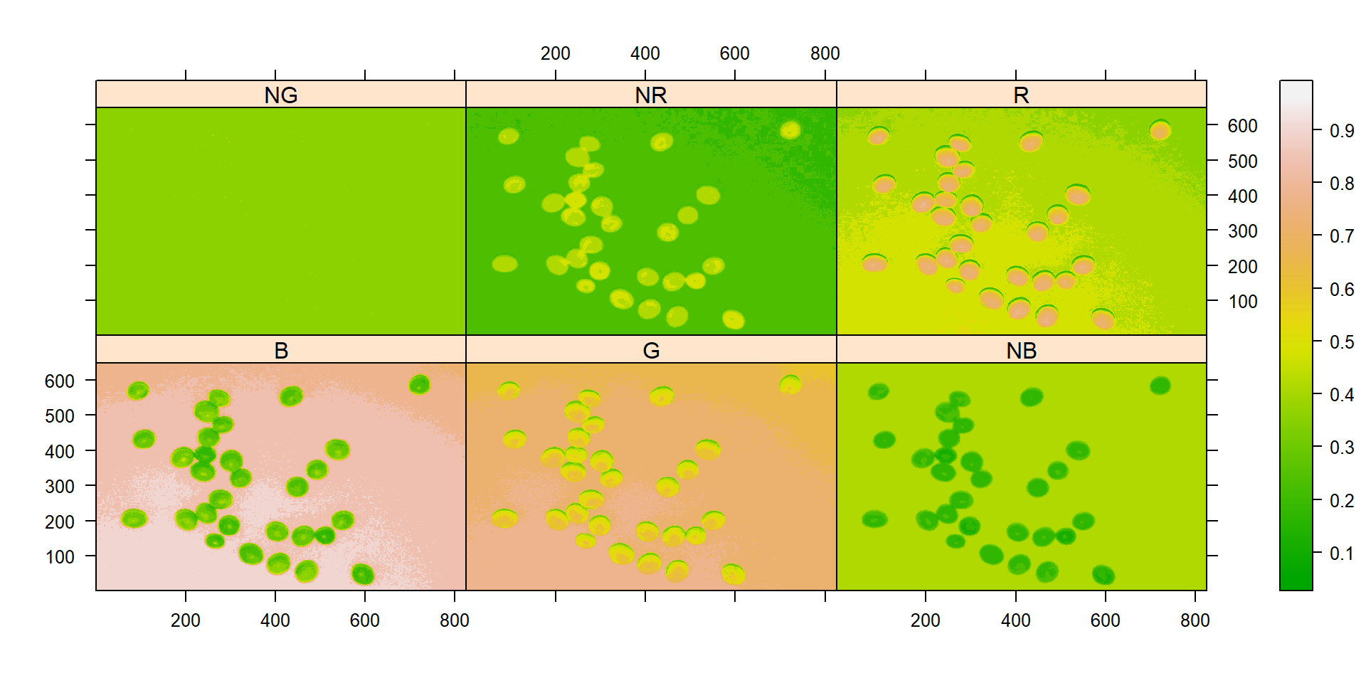
soy <- image_pliman("soybean_touch.jpg")
# Compute the indexes
indexes <- image_index(soy, index = c("R, G, B, NR, NG, NB"))
# Create a raster plot with the RGB values
plot(indexes)
# Create a density plot with the RGB values
plot(indexes, type = "density")
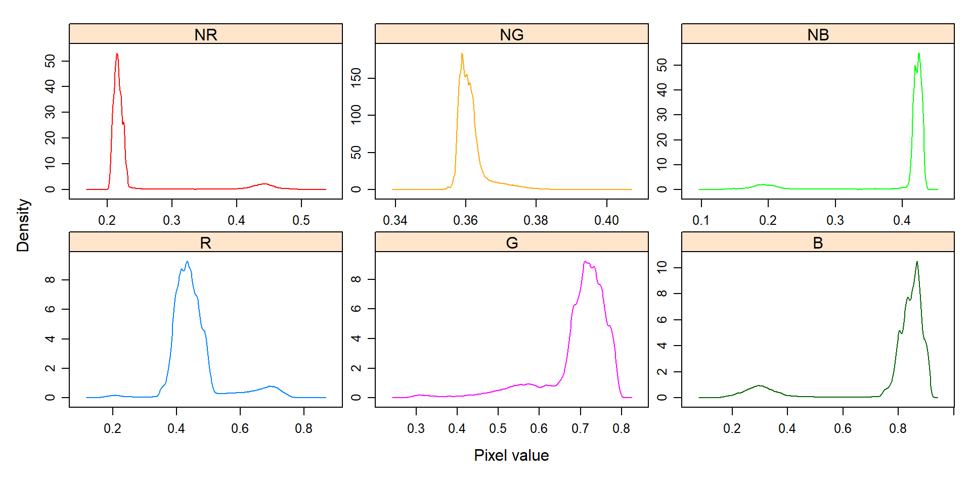
In this example, we can see the distribution of the RGB values (first row) and the normalized RGB values (second row). The two peaks represent the grains (smaller peak) and the blue background (larger peak). The clearer the difference between these peaks, the better will the image segmentation.
Segment an image
The function image_segmentation() is used to segment images using image indexes. In this example, I will use the same indexes computed below to see how the image is segmented. The output of this function can be used as input in the function analyze_objects().
segmented <- image_segment(soy, index = c("R, G, B, NR, NG, NB"))
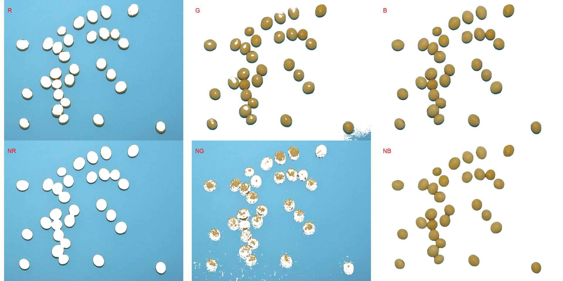
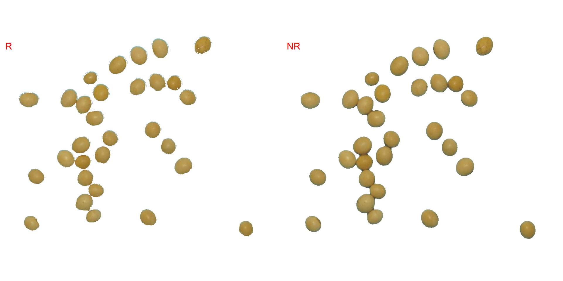
It seems that the "NB" index provided better segmentation. "R" and "NR" resulted in an inverted segmented image, i.e., the grains were considered as background and the remaining as ‘selected’ image. To circumvent this problem, we can use the argument invert in those functions.
image_segment(soy,
              index = c("R, NR"),
              invert = TRUE)
Produce a binary image
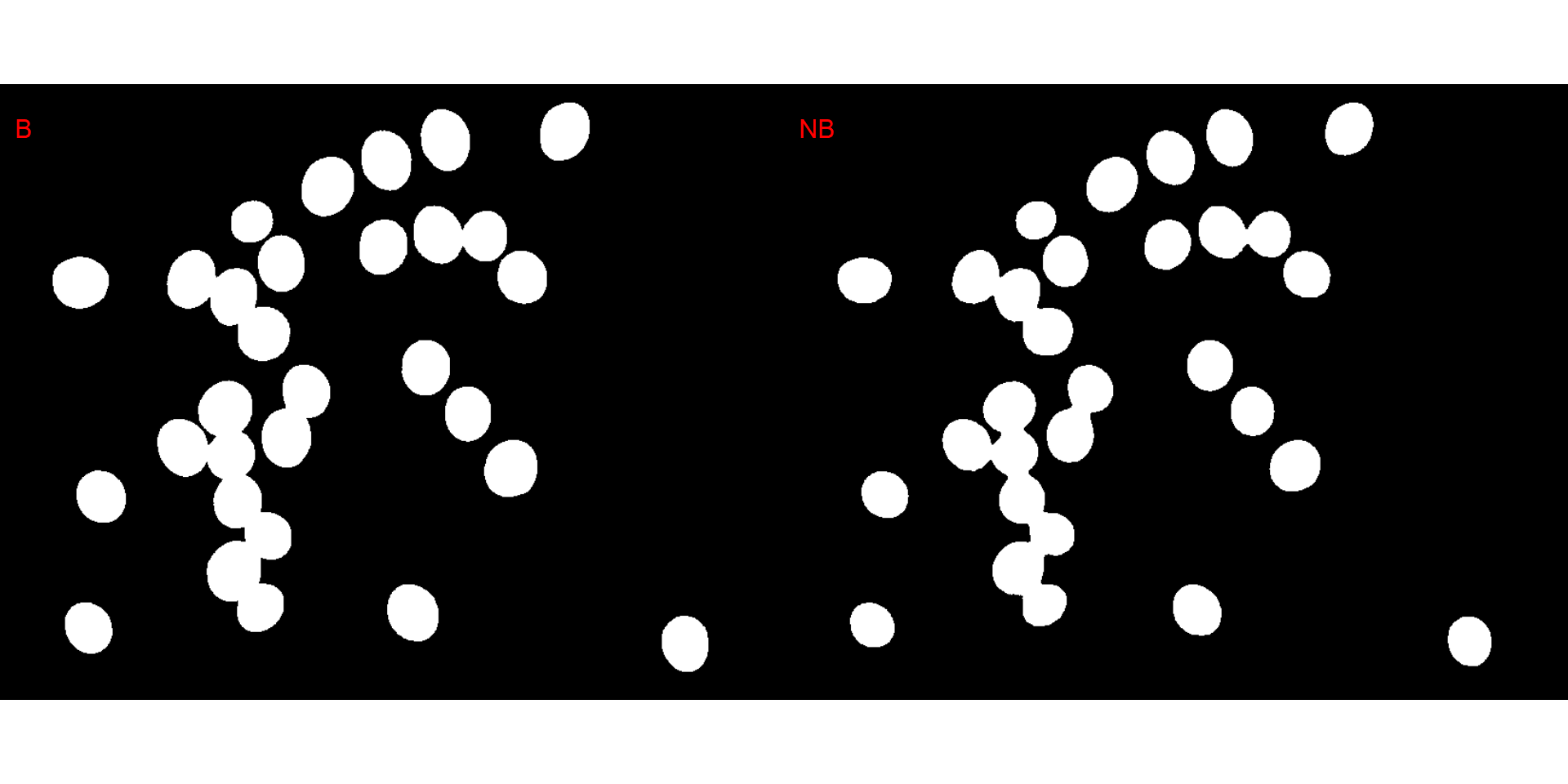
We can also produce a binary image with image_binary(). Just for curiosity, we will use the indexes "B" (blue) and "NB" (normalized blue). By default, image_binary() rescales the image to 30% of the size of the original image to speed up the computation time. Use the argument resize = FALSE to produce a binary image with the original size.
binary <- image_binary(soy)
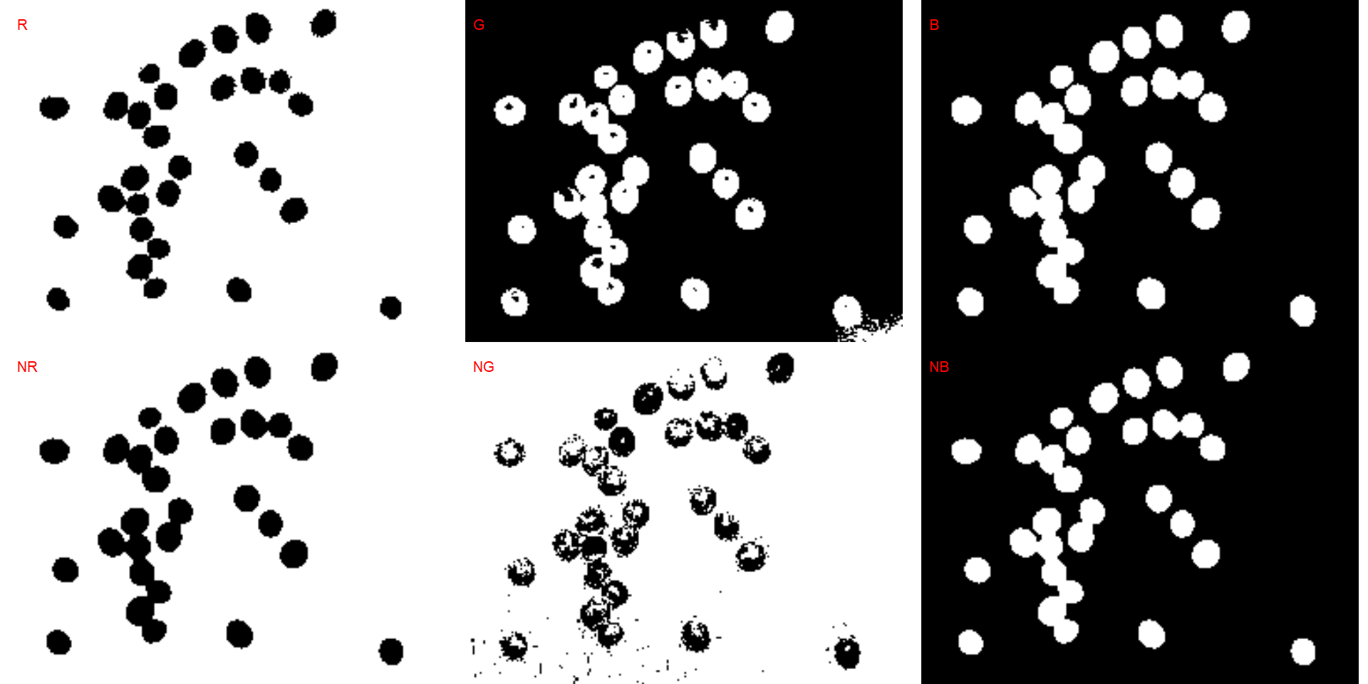
# original image size
image_binary(soy,
             index = c("B, NB"),
             resize = FALSE)
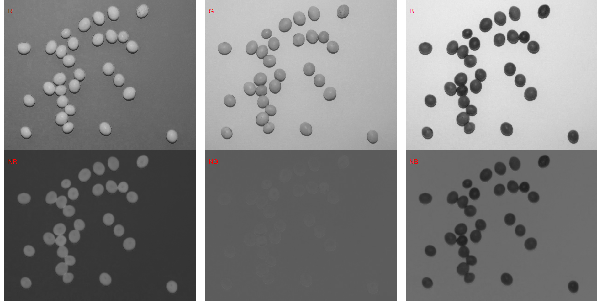
Counting crop grains
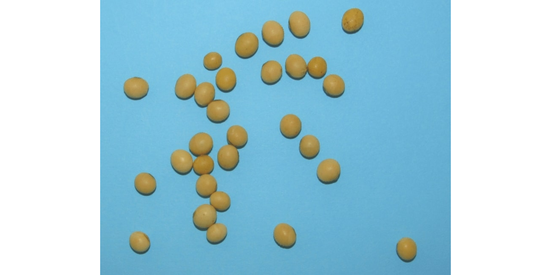
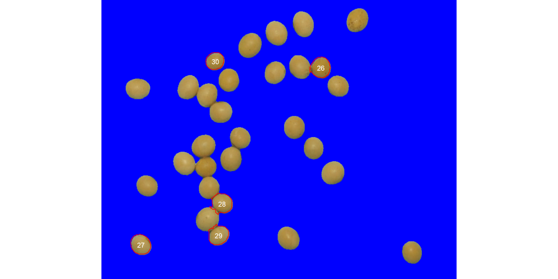
Here, we will count the grains in the image soybean_touch.jpg. This image has a cyan background and contains 30 soybean grains that touch with each other. Two segmentation strategies are used. The first one is by using is image segmentation based on color indexes.
library(pliman)
soy <- image_pliman("soybean_touch.jpg", plot = TRUE)
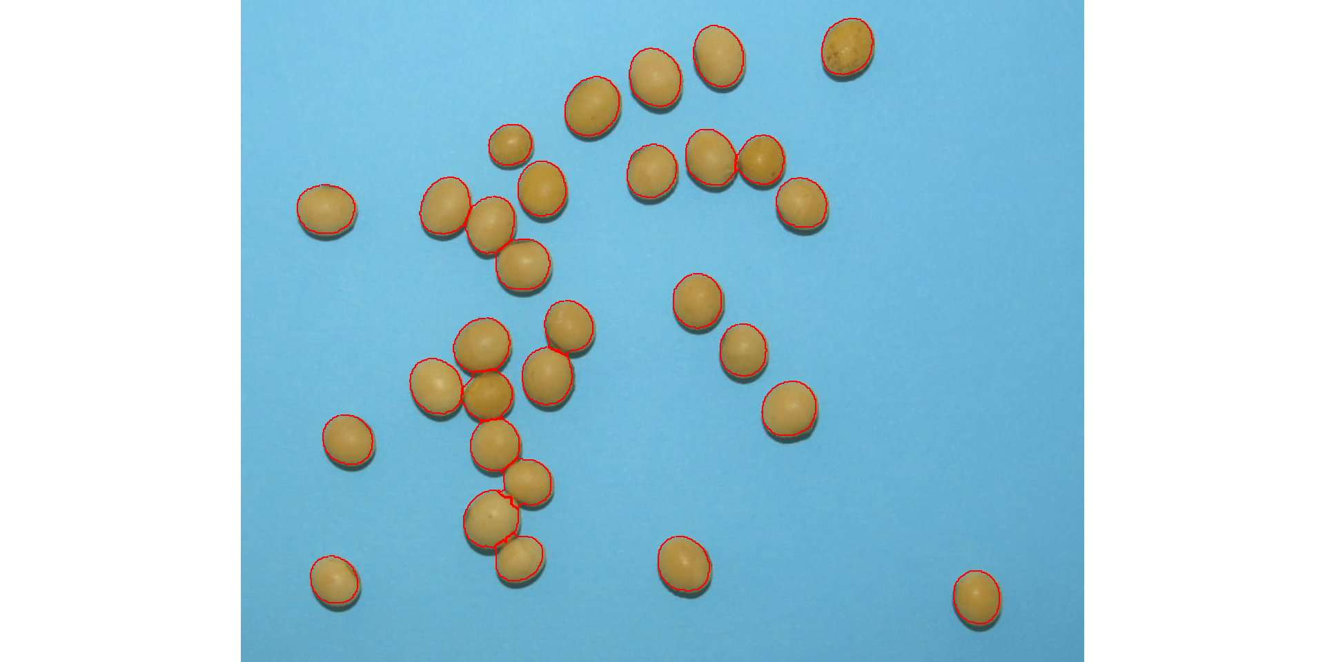
The function analyze_objects() segment the image using as default the normalized blue index, as follows (NB = (B/(R+G+B))), where R, G, and B are the red, green, and blue bands. Objects are counted and the segmented objects are colored with random permutations.
count <-
  analyze_objects(soy,
                  index = "NB") # default
count$statistics
#        stat      value
# 1         n    30.0000
# 2  min_area  1366.0000
# 3 mean_area  2057.3667
# 4  max_area  2445.0000
# 5   sd_area   230.5574
# 6  sum_area 61721.0000
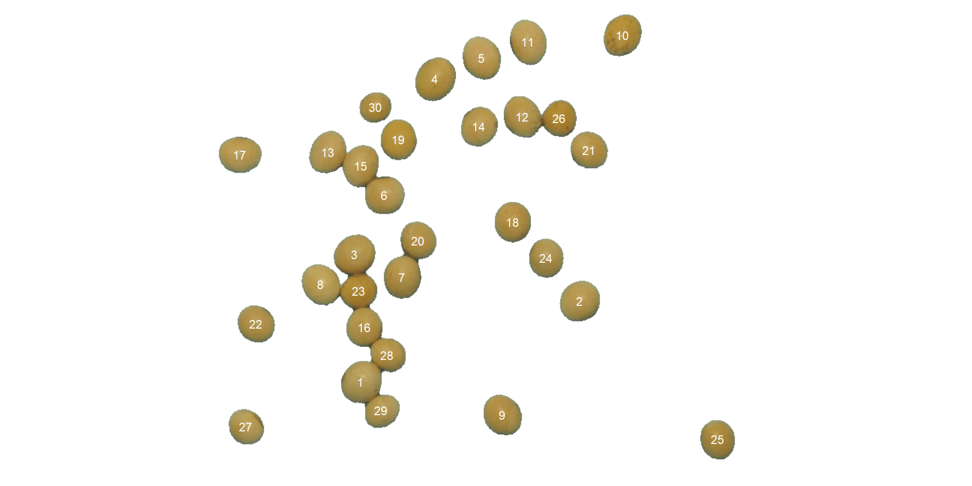
Users can set show_contour = FALSE to remove the contour line and identify the objects (in this example the grains) by using the arguments marker = "id". The color of the background can also be changed with col_background.
count <-
  analyze_objects(soy,
                  show_contour = FALSE,
                  marker = "id",
                  show_segmentation = FALSE,
                  col_background = "white",
                  index = "NB") # default
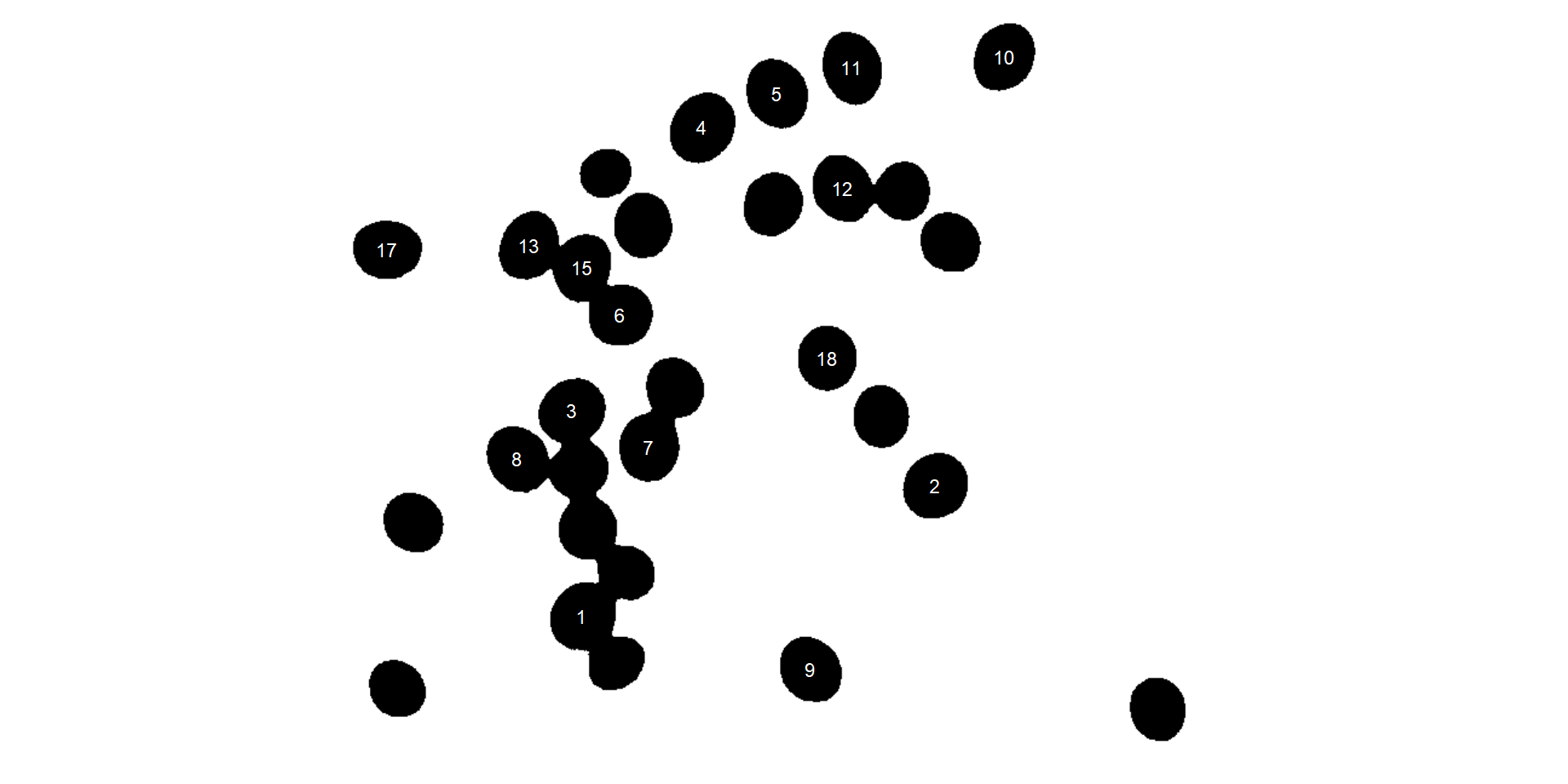
 In the following example, I will select objects with an area above the average of all objects by using
 lower_size = 2057.36. Additionally, I will use the argument show_original = FALSE to show the results as colors (non-original image).
analyze_objects(soy,
                marker = "id",
                show_original = FALSE,
                lower_size = 2057.36,
                index = "NB") # default
Users can also use the topn_* arguments to select the top n objects based on either smaller or largest areas. Let’s see how to point out the 5 grains with the smallest area, showing the original grains in a blue background. We will also use the argument my_index to choose a personalized index to segment the image. Just for comparison, we will set up explicitly the normalized blue index by calling my_index = "B/(R+G+B)".
analyze_objects(soy,
                marker = "id",
                topn_lower = 5,
                col_background = "blue",
                my_index = "B/(R+G+B)") # default
Leaf area
We can use analyze_objects() to compute object features such as area, perimeter, radius, etc. This can be used, for example, to compute leaf area.
Let’s compute the leaf area of leaves with analyze_objects(). First, we use image_segmentation() to identify candidate indexes to segment foreground (leaves) from background.
path <- "https://raw.githubusercontent.com/TiagoOlivoto/paper_pliman/master/data/leaf_area/leaves2.jpg"
leaves <- image_import(path, plot = TRUE)
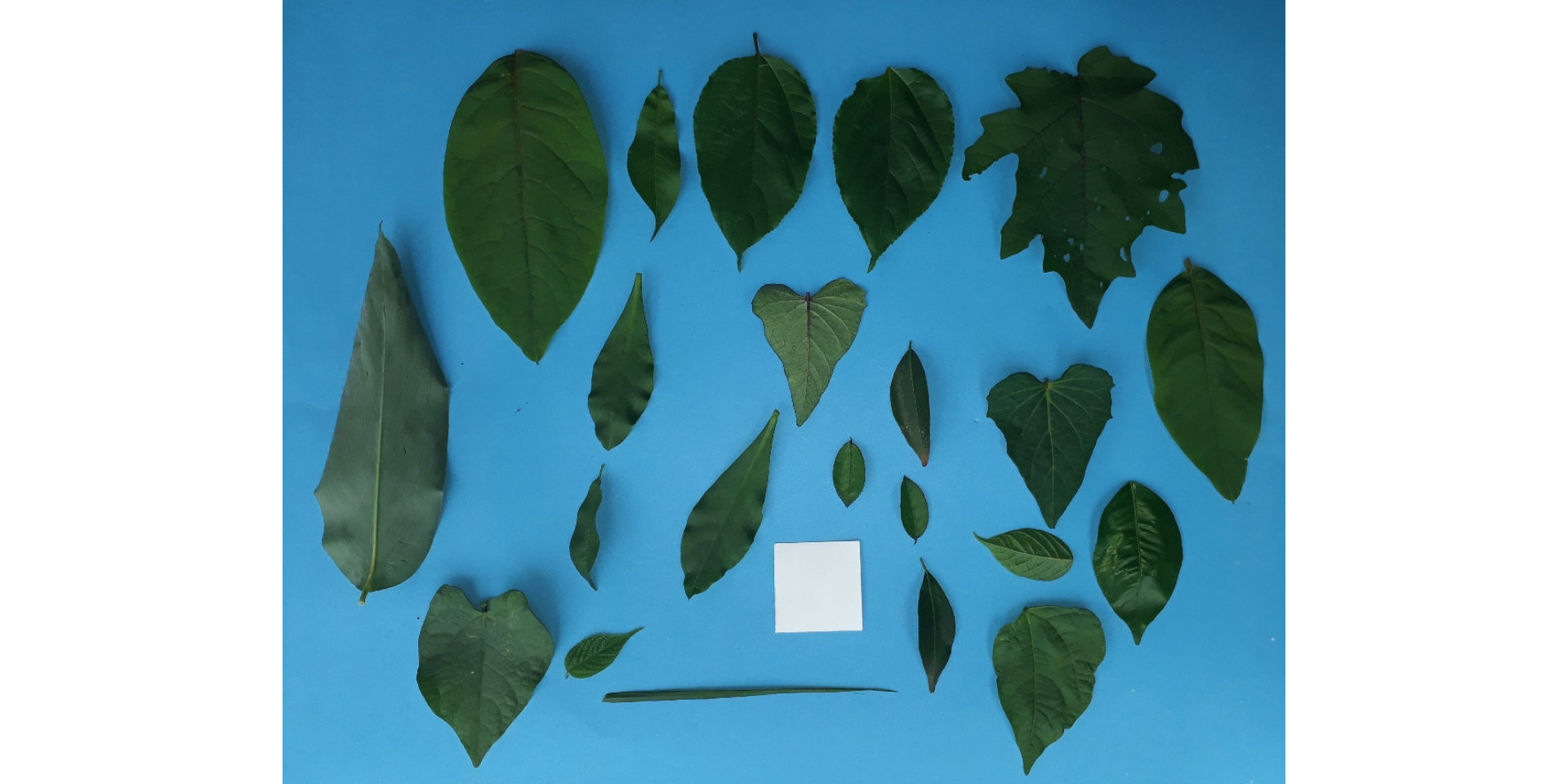
image_segment(leaves, index = "all")
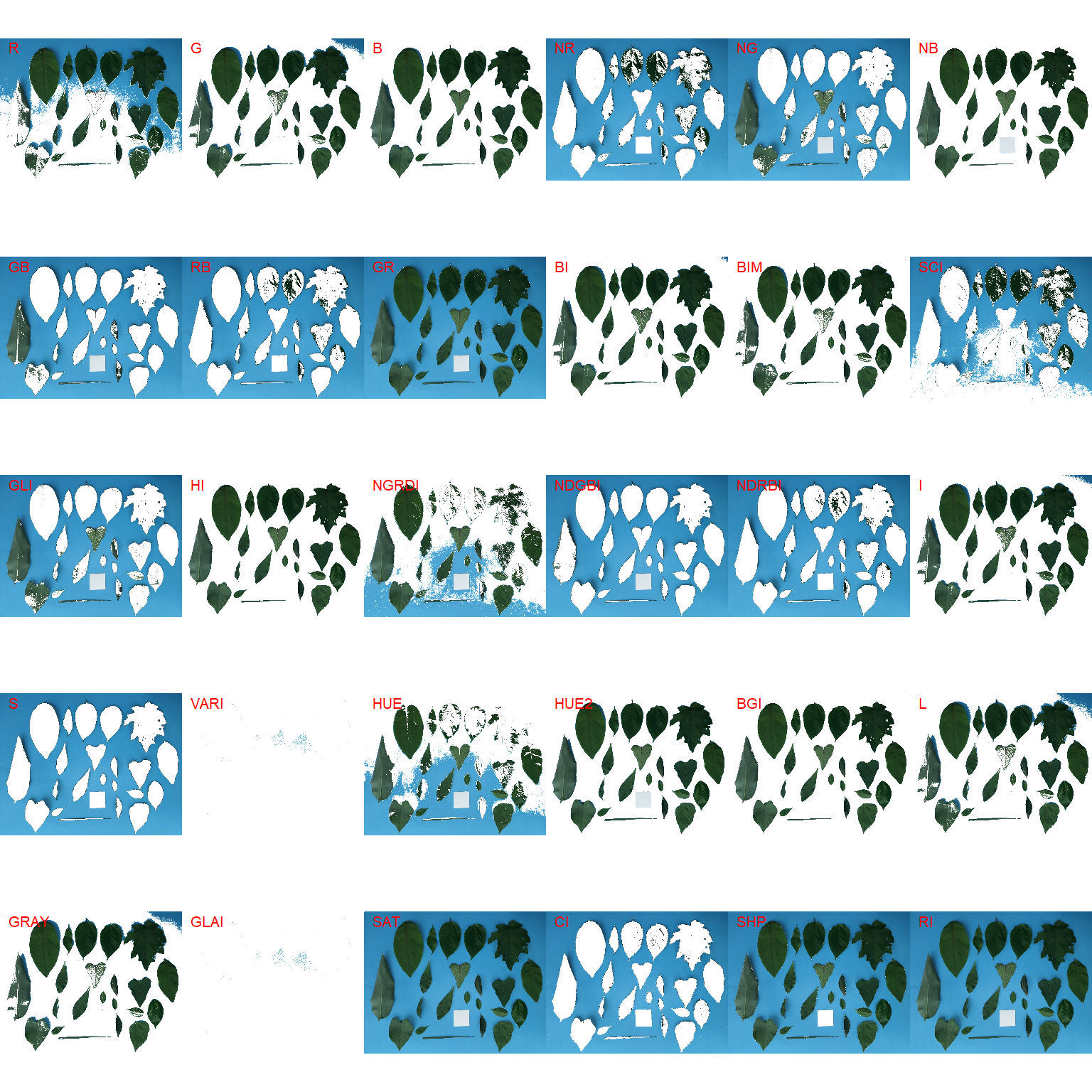
G (Green) and NB (Normalized Blue) are two possible candidates to segment the leaves from the background. We will use the NB index here (default option in analyze_objects()). The measurement of the leaf area in this approach can be done in two main ways: 1) using an object of known area, and 2) knowing the image resolution in dpi (dots per inch).
Using an object of known area
- Count the number of objects (leaves in this case)
Here, we use the argument marker = "id" of the function analyze_objects() to obtain the identification of each object (leaf), allowing for further adjustment of the leaf area. The argument watershed = FALSE is also used to prevent leaves to be segmented into multiple, small fractions.
count <- analyze_objects(leaves,
                         marker = "id",
                         watershed = FALSE)
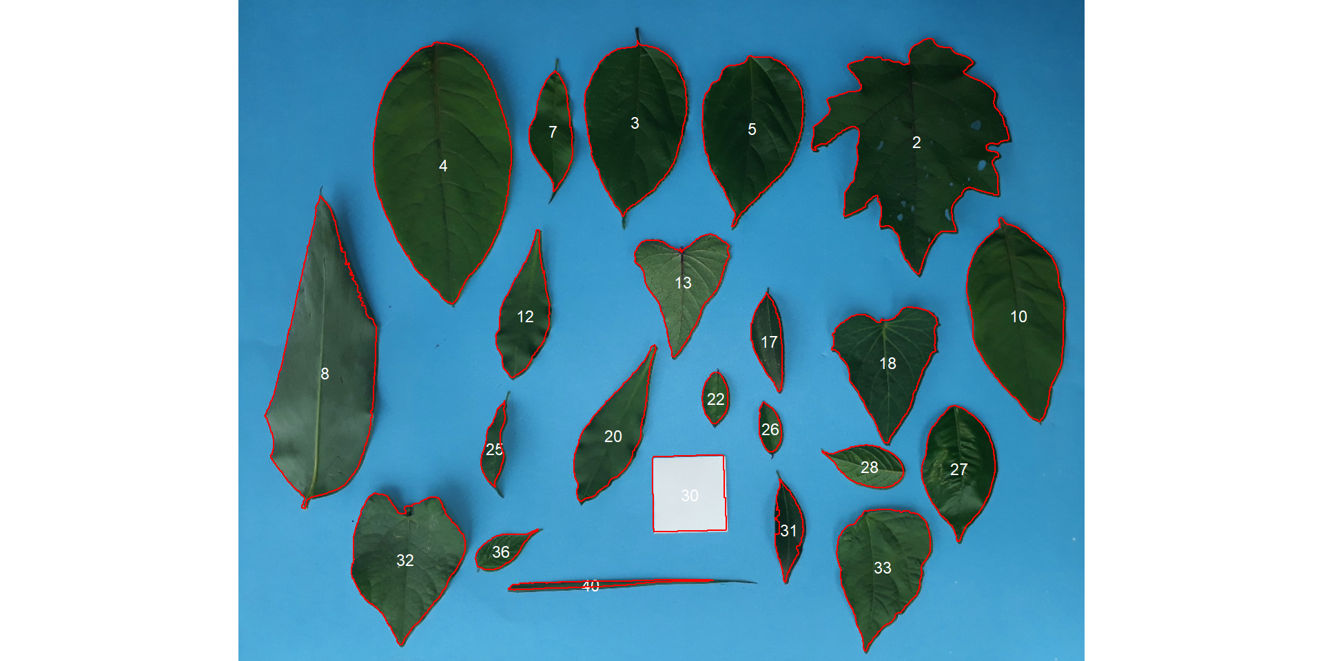
And here we are! Now, all leaves were identified correctly, but all measures were given in pixel units. The next step is to convert these measures to metric units.
- Convert the leaf area by the area of the known object
The function get_measures() is used to adjust the leaf area using object 30, a square with a side of 5 cm (25 cm$^2$).
area <-
  get_measures(count,
               id = 30,
               area ~ 25)
# -----------------------------------------
# measures corrected with:
# object id: 30
# area     : 25
# -----------------------------------------
# Total    : 820.525
# Average  : 35.675
# -----------------------------------------

# plot the area to the segmented image
image_segment(leaves, index = "NB", verbose = FALSE)
plot_measures(area,
              measure = "area",
              col = "red") # default is "white"
knowing the image resolution in dpi (dots per inch)
When the image resolution is known, the measures in pixels obtained with analyze_objects() are corrected by the image resolution. The function dpi() can be used to compute the dpi of an image, provided that the size of any object is known. In this case, the estimated resolution considering the calibration of object 30 was ~50.8 DPIs. We inform this value in the dpi argument of get_measures9).
area2 <- get_measures(count, dpi = 50.8)
# compute the difference between the two methods
sum(area$area - area2$area)
# [1] 7.709
Leaf shape
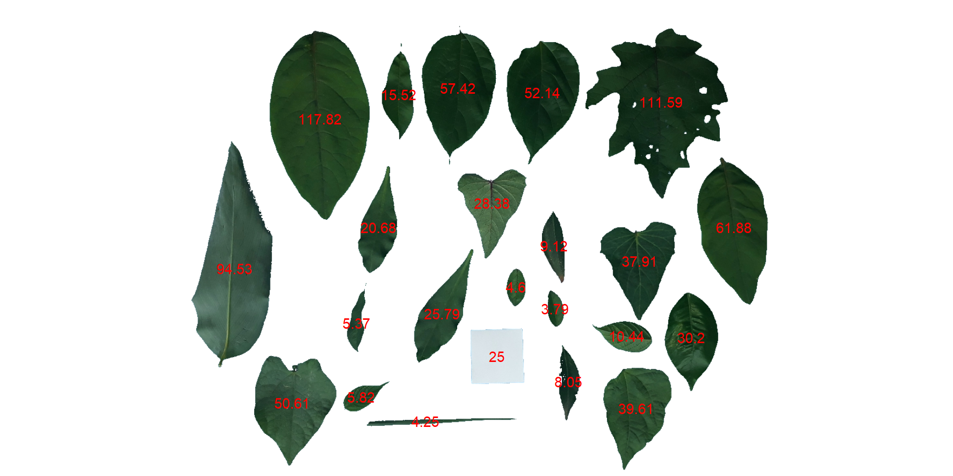
The function analyze_objects() computes a range of object features that can be used to study leaf shape. As a motivating example, I will use the image potato_leaves.png, which was gathered from Gupta et al. (2020)^[Gupta, S., Rosenthal, D. M., Stinchcombe, J. R., & Baucom, R. S. (2020). The remarkable morphological diversity of leaf shape in sweet potato (Ipomoea batatas): the influence of genetics, environment, and G×E. New Phytologist, 225(5), 2183–2195. https://doi.org/10.1111/nph.16286]
potato <- image_pliman("potato_leaves.jpg", plot = TRUE)
pot_meas <-
  analyze_objects(potato,
                  watershed = FALSE,
                  marker = "id",
                  show_chull = TRUE) # shows the convex hull
print(pot_meas$results)
#   id        x        y  area area_ch perimeter radius_mean radius_min
# 1  1 854.5424 224.0429 51380   54536       852    131.5653   92.11085
# 2  2 197.8440 217.8508 58923   76706      1064    140.2962   70.10608
# 3  3 536.2100 240.2380 35117   62792      1310    109.9000   38.13658
#   radius_max radius_sd radius_ratio diam_mean  diam_min diam_max major_axis
# 1   198.0248  26.06131     2.149854  263.1305 184.22169 396.0497   305.7374
# 2   192.3613  28.58523     2.743861  280.5924 140.21215 384.7226   318.2436
# 3   188.5105  35.50978     4.943037  219.8001  76.27315 377.0210   253.4985
#   minor_axis eccentricity      theta  solidity circularity
# 1   242.2124    0.6102310  1.3936873 0.9421300   0.8894566
# 2   274.1280    0.5079648 -0.0992339 0.7681668   0.6540508
# 3   243.2790    0.2810738  1.0968854 0.5592591   0.2571489
Three key measures (in pixel units) are:
areathe area of the object.area_chthe area of the convex hull.perimeterthe perimeter of the object.
Using these measures, circularity and solidity are computed as shown in (Gupta et al, 2020).
$$ circularity = 4\pi(area / perimeter^2) $$ $$ solidity = area / area_ch $$
Circularity is influenced by serrations and lobing. Solidity is sensitive to leaves with deep lobes, or with a distinct petiole, and can be used to distinguish leaves lacking such structures. Unlike circularity, it is not very sensitive to serrations and minor lobings, since the convex hull remains largely unaffected.
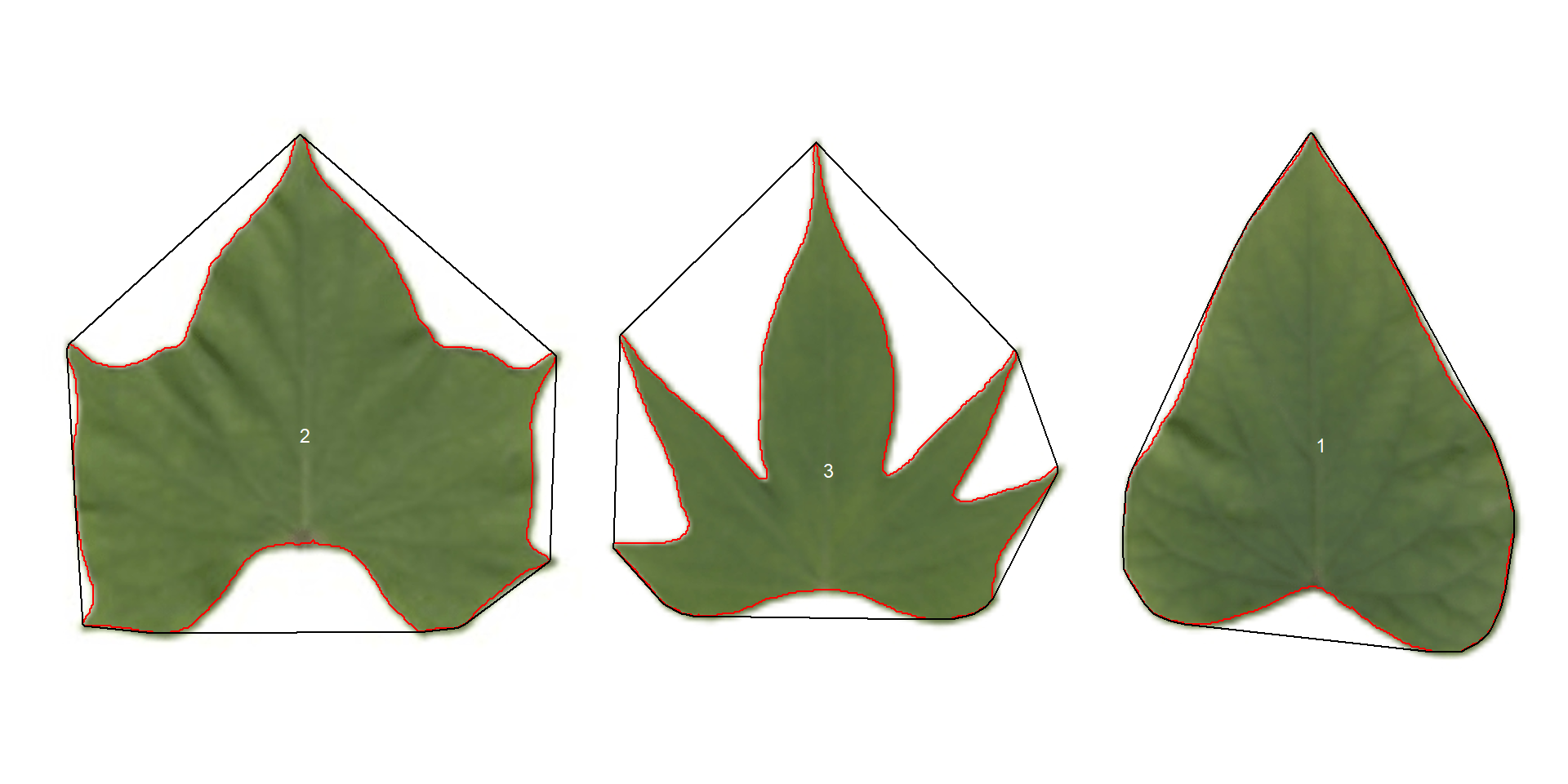
Object contour
Users can also obtain the object contour and convex hull as follows:
cont <-
  object_contour(potato,
                 watershed = FALSE,
                 show_image = FALSE)
plot(potato)
plot_contour(cont, col = "red", lwd = 3)
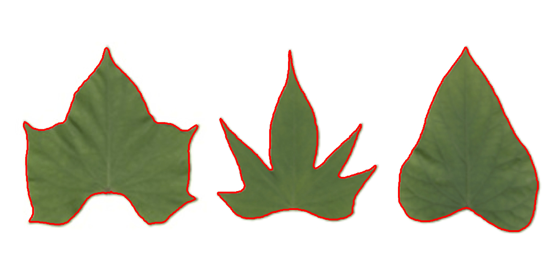
Convex hull
The function object_contour() returns a list with the coordinate points for each object contour that can be further used to obtain the convex hull with conv_hull().
conv <- conv_hull(cont)
plot(potato)
plot_contour(conv, col = "red", lwd = 3)
Area of the convex hull
Then, the area of the convex hull can be obtained with poly_area().
(area <- poly_area(conv))
# $`1`
# [1] 54536
#
# $`2`
# [1] 76706
#
# $`3`
# [1] 62792.5
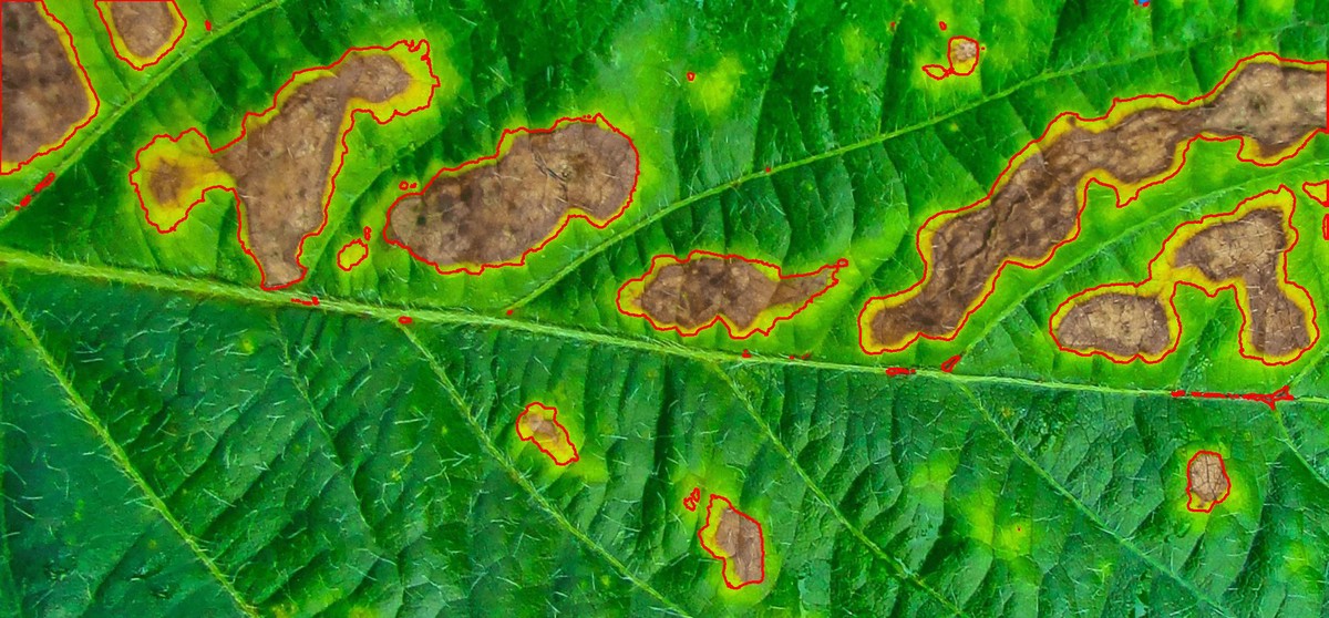
Phytopathometry
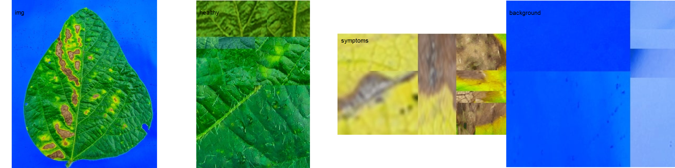
The function measure_disease() can be used to perform phytopathometric studies. A detailed explanation can be seen in the following manuscript.

In brief, users need to provide sample pallets that represent the color classes (healthy, diseased, and background) in the image to be analyzed.
library(pliman)
# set the path directory
path_soy <- "https://raw.githubusercontent.com/TiagoOlivoto/pliman/master/vignettes/imgs"
# import images
img <- image_import("leaf.jpg", path = path_soy)
healthy <- image_import("healthy.jpg", path = path_soy)
symptoms <- image_import("sympt.jpg", path = path_soy)
background <- image_import("back.jpg", path = path_soy)
image_combine(img, healthy, symptoms, background, ncol = 4)
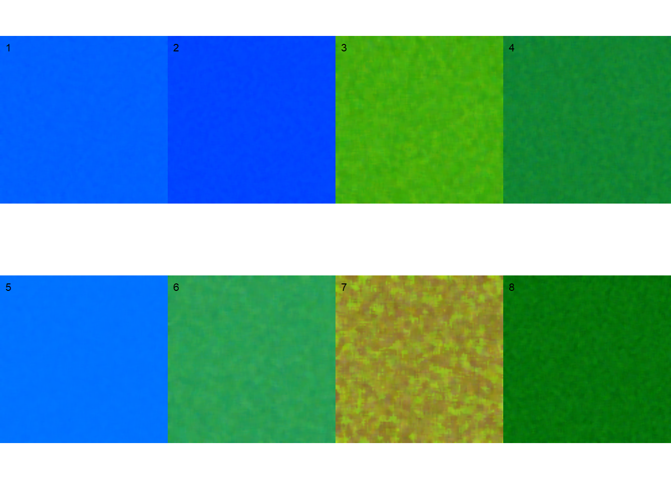
Sample palettes can be made by simply manually sampling small areas of representative images and producing a composite image that will represent each of the desired classes (background, healthy, and symptomatic tissues). Another way is to use the image_palette() function to create sample color palettes
pals <- image_palette(img, npal = 8)
image_combine(pals, ncol = 4)
# default settings
res <-
  measure_disease(img = img,
                  img_healthy = healthy,
                  img_symptoms = symptoms,
                  img_background = background,
                  show_image = FALSE,
                  save_image = TRUE,
                  dir_processed = tempdir())
res$severity
#   healthy symptomatic
# 1 89.4991     10.5009
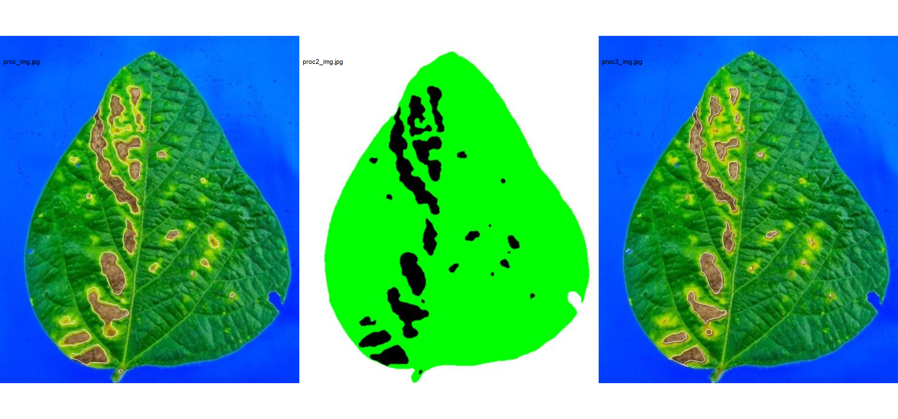
Alternatively, users can create a mask instead of showing the original image.
# create a personalized mask
res2 <-
  measure_disease(img = img,
                  img_healthy = healthy,
                  img_symptoms = symptoms,
                  img_background = background,
                  show_original = FALSE, # create a mask
                  show_contour = FALSE, # hide the contour line
                  col_background = "white", # default
                  col_lesions = "black", # default
                  col_leaf = "green",
                  show_image = FALSE,
                  save_image = TRUE,
                  dir_processed = tempdir(),
                  prefix = "proc2_")

res2$severity
#    healthy symptomatic
# 1 89.13278    10.86722
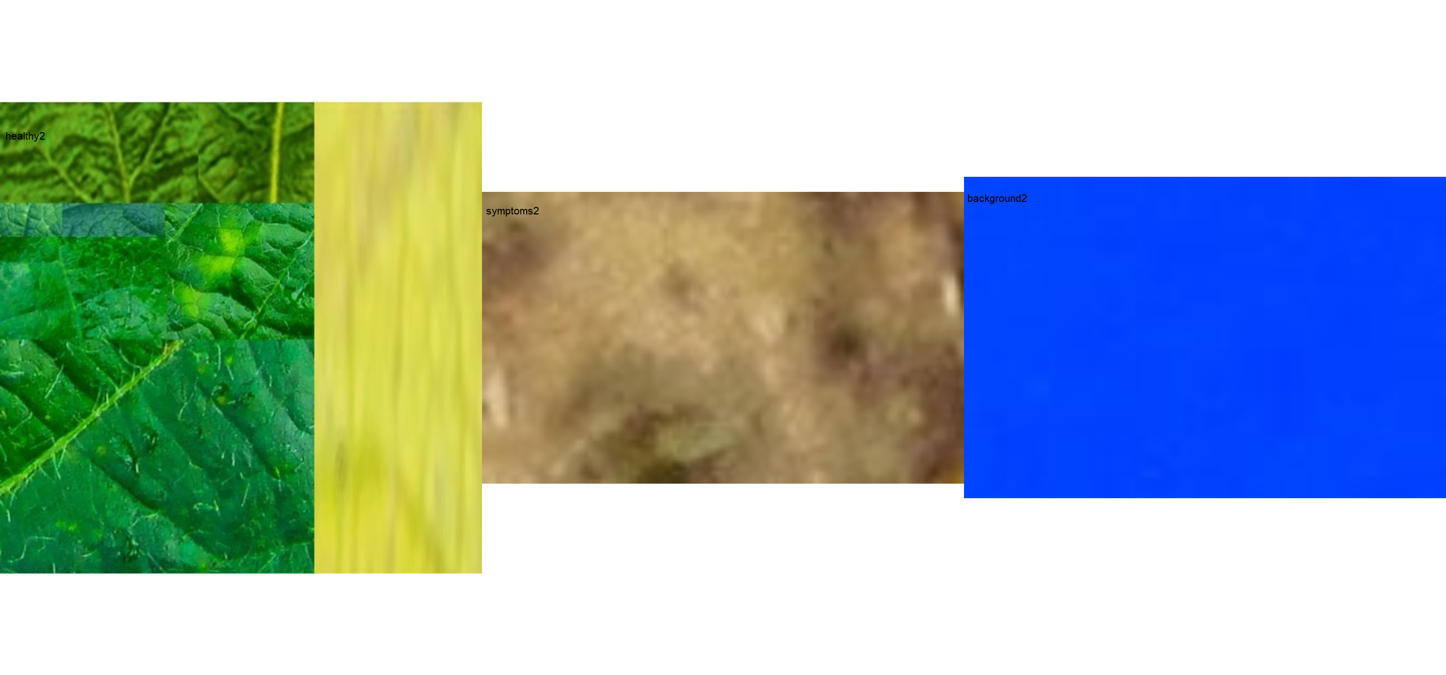
The results may vary depending on how palettes are chosen and are subjective due to the researcher’s experience. In the following example, I show a second example with a variation in the color palettes, where only the necrotic area is assumed to be the diseased tissue. Therefore, the symptomatic area will be smaller than the previous one.
# import images
healthy2 <- image_import("healthy2.jpg", path = path_soy)
symptoms2 <- image_import("sympt2.jpg", path = path_soy)
background2 <- image_import("back2.jpg", path = path_soy)
image_combine(healthy2, symptoms2, background2, ncol = 3)
res3 <-
  measure_disease(img = img,
                  img_healthy = healthy2,
                  img_symptoms = symptoms2,
                  img_background = background2,
                  show_image = FALSE,
                  save_image = TRUE,
                  dir_processed = tempdir(),
                  prefix = "proc3_")
res3$severity
#    healthy symptomatic
# 1 93.82022    6.179779

# combine the masks
masks <-
  image_import(pattern = "proc",
               path = tempdir(),
               plot = TRUE,
               ncol = 3)
Lesion features
res4 <-
  measure_disease(img = img,
                  img_healthy = healthy,
                  img_symptoms = symptoms,
                  img_background = background,
                  show_features = TRUE,
                  marker = "area")
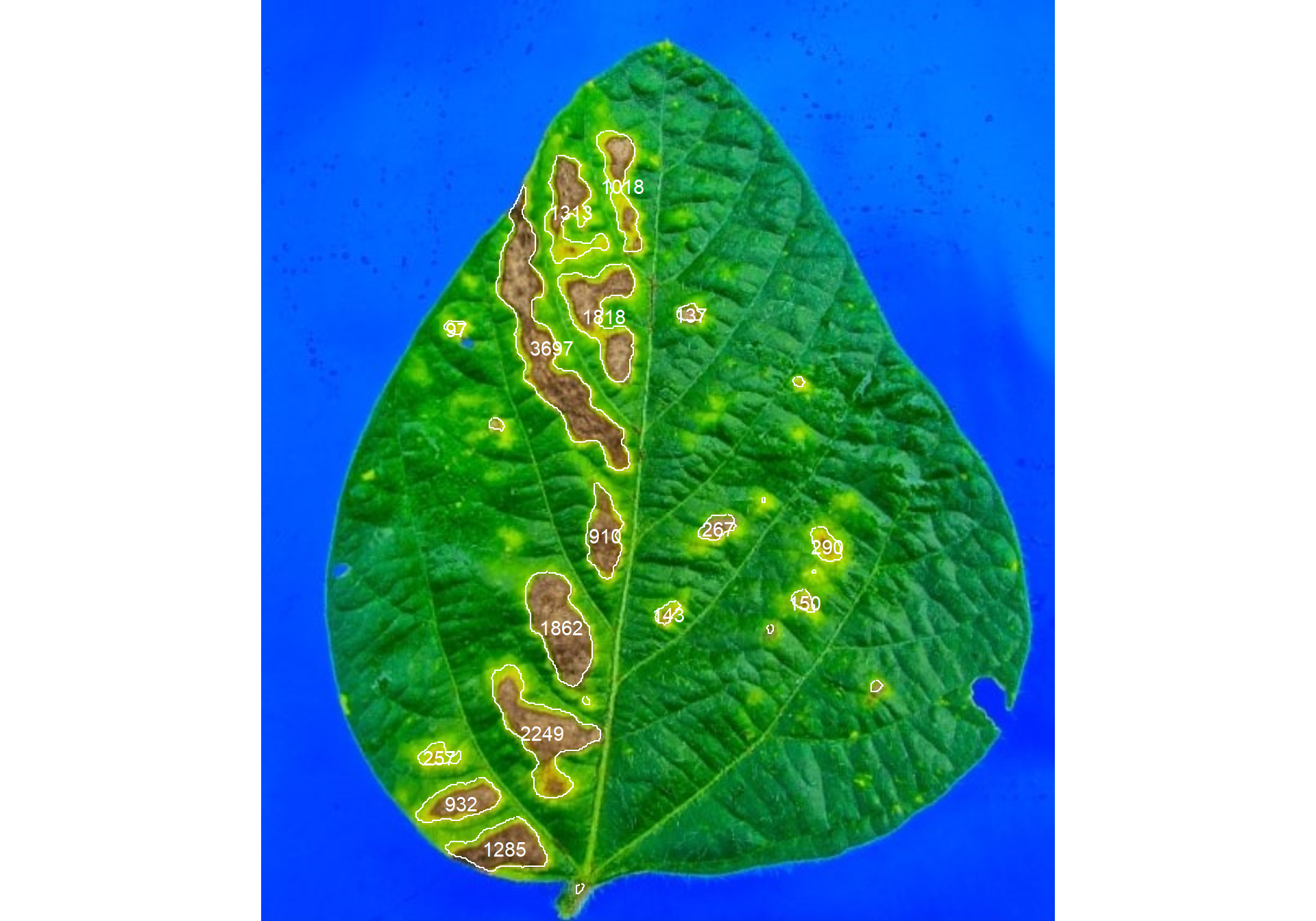
res4$shape
#    id        x        y area perimeter radius_mean radius_min radius_max
# 1   1 222.2859 114.6424 1018       169   22.236026  0.4603231  38.804380
# 2   2 190.7944 130.6923 1313       216   20.505417  1.4443035  38.540057
# 3   3 178.9189 213.9689 3697       402   50.008877  1.8849830  94.905037
# 4   4 210.7998 194.4219 1818       221   24.120230  1.6370150  42.387100
# 5   5 264.3504 193.5839  137        40    6.178002  4.3434577   7.947680
# 6   6 120.4948 202.2990   97        31    5.138492  3.1849019   6.742861
# 9   7 211.8692 329.1473  910       125   18.331786  7.5318035  30.162892
# 11  8 281.2659 325.0037  267        57    9.008080  5.3715448  12.625266
# 12  9 348.0517 335.8966  290        56    9.467631  6.2721546  12.574802
# 14 10 184.7664 385.5258 1862       163   25.072017 12.1560682  38.103388
# 15 11 334.2733 370.1600  150        40    6.599678  4.3102349   9.139372
# 16 12 250.6783 377.3566  143        38    6.528163  3.5109642   9.322329
# 18 13 173.3286 450.2530 2249       240   28.669347 12.6335484  47.607929
# 21 14 110.0817 465.0739  257        65    8.885633  3.5711202  13.781224
# 22 15 123.5966 493.3455  932       114   17.782799  9.5688608  27.515577
# 23 16 149.9315 521.2646 1285       141   21.112364 11.1572209  32.888613
#    radius_sd radius_ratio major_axis eccentricity        theta
# 1  11.188456    84.298141   89.44536    0.9773644  1.397905986
# 2   8.945422    26.684182   72.58292    0.8880396  1.482811710
# 3  25.441561    50.347955  191.01128    0.9783889  1.166481100
# 4  10.107604    25.892921   81.07238    0.8432963  1.276850162
# 5   1.091633     1.829805   16.09211    0.7170820  0.103325743
# 6   1.000345     2.117133   13.64816    0.7240212  0.041687762
# 9   6.398871     4.004737   56.65709    0.9264766  1.537663173
# 11  1.987051     2.350398   24.91008    0.8274979 -0.447328474
# 12  1.933473     2.004862   25.53176    0.8178648  0.964221254
# 14  7.480733     3.134516   75.73913    0.9053726  1.206510884
# 15  1.300432     2.120388   17.32549    0.7498443  0.725329876
# 16  1.623321     2.655205   18.86956    0.8491418 -0.758279140
# 18  9.824264     3.768373   88.76454    0.8546704  0.986657251
# 21  2.877021     3.859076   26.77591    0.8435809  0.009328961
# 22  5.532855     2.875533   54.17616    0.9112499 -0.290029006
# 23  6.003319     2.947742   59.27819    0.8605355 -0.058009041
res4$statistics
#        stat     value
# 1         n    16.000
# 2  min_area    97.000
# 3 mean_area  1026.562
# 4  max_area  3697.000
# 5   sd_area  1001.249
# 6  sum_area 16425.000
A little bit more!
At this link you will find more examples on how to use {pliman} to analyze plant images. Source code and images can be downloaded here.
The following talk (Portuguese language) was ministered to attend the invitation of the President of the Brazilian Region of the International Biometric Society (RBras).