metan 1.16.0 is now available!
 Image by jplenio from Pixabay
After almost four months since the last stable release, I’m so proud to announce that metan 1.16.0 is now on
CRAN. metan was first released on CRAN on 2020/01/14 and since there, 13 stable versions have been released regularly. This new version includes new features and bug corrections. In the last months, I’ve been receiving a lot of positive feedbacks and very useful suggestions to improve the package. Thanks to all!
Instalation
# The latest stable version is installed with
install.packages("metan")

# Or the development version from GitHub:
# install.packages("devtools")
devtools::install_github("TiagoOlivoto/metan")
New features
AMMI indexes
In this version, new AMMI-stability methods were included in ammi_indexes().
- AMMI Based Stability Parameter (ASTAB) (Rao and Prabhakaran 2005)
$$ ASTAB = \sum_{n=1}^{N’}\lambda_{n}\gamma_{in}^{2} $$
-
AMMI Stability Index (ASI) (Jambhulkar et al. 2017) $$ ASI = \sqrt{\left [PC_{1}^{2} \times \theta_{1}^{2} \right ]+\left[ PC_{2}^{2} \times \theta_{2}^{2} \right ]} $$
-
AMMI-stability value (ASV) (Purchase et al., 2000) $$ ASV_{i}=\sqrt{\frac{SS_{IPCA1}}{SS_{IPCA2}}(\mathrm{IPC} \mathrm{A} 1)^{2}+(\mathrm{IPCA} 2)^{2}} $$
-
Sum Across Environments of Absolute Value of GEI Modelled by AMMI (AVAMGE) (Zali et al. 2012) $$ AV_{(AMGE)} = \sum_{j=1}^{E} \sum_{n=1}^{N’} \left |\lambda_{n}\gamma_{in} \delta_{jn} \right | $$
-
Annicchiarico’s D Parameter values (Da) (Annicchiarico 1997) $$ D_{a} = \sqrt{\sum_{n=1}^{N’}(\lambda_{n}\gamma_{in})^2} $$
-
Zhang’s D Parameter (Dz) (Zhang et al. 1998) $$ D_{z} = \sqrt{\sum_{n=1}^{N’}\gamma_{in}^{2}} $$
-
Sums of the Averages of the Squared Eigenvector Values (EV) (Zobel 1994) $$ EV = \sum_{n=1}^{N’}\frac{\gamma_{in}^2}{N’} $$
-
Stability Measure Based on Fitted AMMI Model (FA) (Raju 2002) $$ FA = \sum_{n=1}^{N’}\lambda_{n}^{2}\gamma_{in}^{2} $$
-
Modified AMMI Stability Index (MASI) (Ajay et al. 2018) $$ MASI = \sqrt{ \sum_{n=1}^{N’} PC_{n}^{2} \times \theta_{n}^{2}} $$
-
Modified AMMI Stability Value (MASV) (Ajay et al. 2019) $$ MASV = \sqrt{\sum_{n=1}^{N’-1}\left (\frac{SSIPC_{n}}{SSIPC_{n+1}} \right ) \times (PC_{n})^2 + \left (PC_{N’}\right )^2} $$
-
Sums of the Absolute Value of the IPC Scores (SIPC) (Sneller et al. 1997) $$ SIPC = \sum_{n=1}^{N’} | \lambda_{n}^{0.5}\gamma_{in}| $$
-
Absolute Value of the Relative Contribution of IPCs to the Interaction (Za) (Zali et al. 2012) $$ Za = \sum_{i=1}^{N’} | \theta_{n}\gamma_{in} | $$
-
Weighted average of absolute scores (WAAS) (Olivoto et al. 2019) $$ WAAS_i = \sum_{k = 1}^{p} |IPCA_{ik} \times \theta_{k}/ \sum_{k = 1}^{p}\theta_{k} $$
For all the statistics, simultaneous selection indexes (SSI) are also computed by summation of the ranks of the stability and mean performance, Y_R, (Farshadfar, 2008).
library(metan)
# Registered S3 method overwritten by 'GGally':
#   method from
#   +.gg   ggplot2
# |=========================================================|
# | Multi-Environment Trial Analysis (metan) v1.16.0        |
# | Author: Tiago Olivoto                                   |
# | Type 'citation('metan')' to know how to cite metan      |
# | Type 'vignette('metan_start')' for a short tutorial     |
# | Visit 'https://bit.ly/pkgmetan' for a complete tutorial |
# |=========================================================|
model <-
  performs_ammi(data_ge,
                env = ENV,
                gen = GEN,
                rep = REP,
                resp = c(GY, HM),
                verbose = FALSE)
model_indexes <- ammi_indexes(model)
rbind_fill_id(model_indexes, .id = "TRAIT")
# # A tibble: 20 x 43
#    TRAIT GEN       Y   Y_R  ASTAB ASTAB_R ssiASTAB    ASI ASI_R ASI_SSI   ASV
#    <chr> <chr> <dbl> <dbl>  <dbl>   <dbl>    <dbl>  <dbl> <dbl>   <dbl> <dbl>
#  1 GY    G1     2.60     6 0.108        2        8 0.110      4      10 0.346
#  2 GY    G10    2.47    10 1.47        10       20 0.389     10      20 1.23
#  3 GY    G2     2.74     3 0.820        7       10 0.0792     2       5 0.249
#  4 GY    G3     2.96     2 0.0959       1        3 0.0359     1       3 0.113
#  5 GY    G4     2.64     5 0.363        4        9 0.189      7      12 0.594
#  6 GY    G5     2.54     7 0.259        3       10 0.137      5      12 0.430
#  7 GY    G6     2.53     8 0.440        6       14 0.0843     3      11 0.265
#  8 GY    G7     2.74     4 0.971        9       13 0.211      8      12 0.663
#  9 GY    G8     3.00     1 0.416        5        6 0.182      6       7 0.574
# 10 GY    G9     2.51     9 0.947        8       17 0.312      9      18 0.983
# 11 HM    G1    47.1      9 3.49         5       14 0.166      2      11 0.571
# 12 HM    G10   48.5      4 7.51        10       14 0.819     10      14 2.83
# 13 HM    G2    46.7     10 5.35         8       18 0.564      8      18 1.95
# 14 HM    G3    47.6      8 2.86         3       11 0.132      1       9 0.455
# 15 HM    G4    48.0      5 4.26         6       11 0.538      7      12 1.86
# 16 HM    G5    49.3      1 6.35         9       10 0.623      9      10 2.15
# 17 HM    G6    48.7      3 2.22         1        4 0.202      3       6 0.698
# 18 HM    G7    48.0      6 3.39         4       10 0.443      6      12 1.53
# 19 HM    G8    49.1      2 2.42         2        4 0.360      4       6 1.24
# 20 HM    G9    47.9      7 4.36         7       14 0.372      5      12 1.28
# # ... with 32 more variables: ASV_R <dbl>, ASV_SSI <dbl>, AVAMGE <dbl>,
# #   AVAMGE_R <dbl>, AVAMGE_SSI <dbl>, DA <dbl>, DA_R <dbl>, DA_SSI <dbl>,
# #   DZ <dbl>, DZ_R <dbl>, DZ_SSI <dbl>, EV <dbl>, EV_R <dbl>, EV_SSI <dbl>,
# #   FA <dbl>, FA_R <dbl>, FA_SSI <dbl>, MASI <dbl>, MASI_R <dbl>,
# #   MASI_SSI <dbl>, MASV <dbl>, MASV_R <dbl>, MASV_SSI <dbl>, SIPC <dbl>,
# #   SIPC_R <dbl>, SIPC_SSI <dbl>, ZA <dbl>, ZA_R <dbl>, ZA_SSI <dbl>,
# #   WAAS <dbl>, WAAS_R <dbl>, WAAS_SSI <dbl>
Mean performance and stability
It is now possible to perform the weighting process between mean performance and stability using a model computed with mps(). The main difference is that with mps() users can choose among several stability measures, different than waasb().
# using the default values
# WAASB for stability
# BLUP for mean performance
model <-
  mps(data_ge,
      env = ENV,
      gen = GEN,
      rep = REP,
      resp = everything())
# Evaluating trait GY |======================                      | 50% 00:00:01
Evaluating trait HM |============================================| 100% 00:00:02
# Method: REML/BLUP
# Random effects: GEN, GEN:ENV
# Fixed effects: ENV, REP(ENV)
# Denominador DF: Satterthwaite's method
# ---------------------------------------------------------------------------
# P-values for Likelihood Ratio Test of the analyzed traits
# ---------------------------------------------------------------------------
#     model       GY       HM
#  COMPLETE       NA       NA
#       GEN 1.11e-05 5.07e-03
#   GEN:ENV 2.15e-11 2.27e-15
# ---------------------------------------------------------------------------
# All variables with significant (p < 0.05) genotype-vs-environment interaction
# Mean performance: blupg
# Stability: waasb
model$mps_ind
# # A tibble: 10 x 3
#    GEN      GY    HM
#    <chr> <dbl> <dbl>
#  1 G1     57.6  56.2
#  2 G10     0    35.0
#  3 G2     59.9  17.8
#  4 G3     95.5  67.9
#  5 G4     45.7  58.6
#  6 G5     40.0  61.1
#  7 G6     45.9  85.5
#  8 G7     45.2  51.3
#  9 G8     77.3  90.6
# 10 G9     16.3  58.7

# Deviations from the Eberhart and Russell regression as stability measure
# Best linear unbiased estimates (BLUE) as mean performance
model2 <-
  mps(data_ge,
      env = ENV,
      gen = GEN,
      rep = REP,
      resp = everything(),
      performance = "blueg",
      stability = "s2di")
# Evaluating trait GY |======================                      | 50% 00:00:00
Evaluating trait HM |============================================| 100% 00:00:01
# Method: REML/BLUP
# Random effects: GEN, GEN:ENV
# Fixed effects: ENV, REP(ENV)
# Denominador DF: Satterthwaite's method
# ---------------------------------------------------------------------------
# P-values for Likelihood Ratio Test of the analyzed traits
# ---------------------------------------------------------------------------
#     model       GY       HM
#  COMPLETE       NA       NA
#       GEN 1.11e-05 5.07e-03
#   GEN:ENV 2.15e-11 2.27e-15
# ---------------------------------------------------------------------------
# All variables with significant (p < 0.05) genotype-vs-environment interaction
# Mean performance: blueg
# Stability: s2di
model2$mps_ind
# # A tibble: 10 x 3
#    GEN      GY    HM
#    <chr> <dbl> <dbl>
#  1 G1     59.4  56.0
#  2 G10     0    35.0
#  3 G2     59.2  19.3
#  4 G3     95.5  67.9
#  5 G4     54.8  53.8
#  6 G5     50.5  68.9
#  7 G6     51.7  88.4
#  8 G7     56.7  58.5
#  9 G8     86.6  88.7
# 10 G9     25.6  68.3


p1 <- wsmp(model) %>% plot()
# Warning: object `x` seems to be computed with `mps()`. Switching to `type = 2`.
# Warning: Vectorized input to `element_text()` is not officially supported.
# Results may be unexpected or may change in future versions of ggplot2.
p2 <- wsmp(model2) %>% plot()
# Warning: object `x` seems to be computed with `mps()`. Switching to `type = 2`.

# Warning: Vectorized input to `element_text()` is not officially supported.
# Results may be unexpected or may change in future versions of ggplot2.
arrange_ggplot(p1, p2)
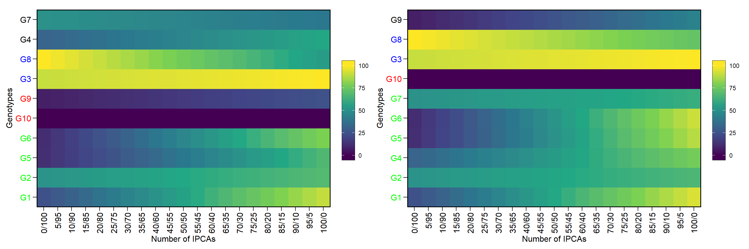
Figure 1: Genotype ranking according to different weights given for mean performance and stability. (a) WAASB x BLUP, (b) s2di x BLUE
ge_stats
ge_stats() now returns
ges <- ge_stats(data_ge2,
                env = ENV,
                gen = GEN,
                rep = REP,
                resp = PH)
# Evaluating trait PH |============================================| 100% 00:00:03
stats <- gmd(ges)
# Class of the model: ge_stats
# Variable extracted: stats
stats
# # A tibble: 13 x 44
#    var   GEN       Y    CV   ACV    POLAR   Var Shukla  Wi_g  Wi_f  Wi_u Ecoval
#    <chr> <chr> <dbl> <dbl> <dbl>    <dbl> <dbl>  <dbl> <dbl> <dbl> <dbl>  <dbl>
#  1 PH    H1     2.62 11.8  12.5  -0.0439  0.286 0.0602  90.2  92.7  89.8  0.493
#  2 PH    H10    2.31 15.2  14.1   0.0603  0.372 0.0301  81.6  91.7  76.1  0.264
#  3 PH    H11    2.39 13.3  12.7  -0.0287  0.301 0.0237  85.8  96.2  80.7  0.215
#  4 PH    H12    2.44 10.4  10.2  -0.220   0.193 0.0769  80.1  93.6  67.0  0.620
#  5 PH    H13    2.54  8.96  9.19 -0.311   0.155 0.0869  82.4  97.7  70.9  0.696
#  6 PH    H2     2.60 13.3  14.1   0.0582  0.362 0.0657  88.5  99.8  86.0  0.535
#  7 PH    H3     2.59 16.6  17.4   0.246   0.558 0.0819  85.8  92.8  77.6  0.659
#  8 PH    H4     2.58 14.8  15.4   0.139   0.436 0.0475  89.2 101.   80.7  0.397
#  9 PH    H5     2.57 12.7  13.2   0.00211 0.319 0.0162  94.1  99.3  87.9  0.158
# 10 PH    H6     2.56 12.0  12.4  -0.0475  0.285 0.0396  90.1  98.4  89.2  0.336
# 11 PH    H7     2.40 12.6  12.2  -0.0672  0.275 0.0272  85.8  98.6  77.7  0.241
# 12 PH    H8     2.33 15.1  14.1   0.0605  0.372 0.0618  77.8  93.0  68.1  0.505
# 13 PH    H9     2.36 16.5  15.7   0.153   0.459 0.0321  83.5  82.8  86.5  0.279
# # ... with 32 more variables: bij <dbl>, Sij <dbl>, R2 <dbl>, ASTAB <dbl>,
# #   ASI <dbl>, ASV <dbl>, AVAMGE <dbl>, DA <dbl>, DZ <dbl>, EV <dbl>, FA <dbl>,
# #   MASI <dbl>, MASV <dbl>, SIPC <dbl>, ZA <dbl>, WAAS <dbl>, WAASB <dbl>,
# #   HMGV <dbl>, RPGV <dbl>, HMRPGV <dbl>, Pi_a <dbl>, Pi_f <dbl>, Pi_u <dbl>,
# #   Gai <dbl>, S1 <dbl>, S2 <dbl>, S3 <dbl>, S6 <dbl>, N1 <dbl>, N2 <dbl>,
# #   N3 <dbl>, N4 <dbl>
Cheatsheet
Citation
To cite metan in your publications, please, use the official reference paper:
Olivoto, T., and Lúcio, A.D. (2020). metan: an R package for multi-environment trial analysis. Methods Ecol Evol. 11:783-789 doi: 10.1111/2041-210X.13384
A BibTeX entry for LaTeX users is
@Article{Olivoto2020,
author = {Tiago Olivoto and Alessandro Dal'Col L{'{u}}cio},
title = {metan: an R package for multi-environment trial analysis},
journal = {Methods in Ecology and Evolution},
volume = {11},
number = {6},
pages = {783-789},
year = {2020},
doi = {10.1111/2041-210X.13384},
}
References
Rao AR, Prabhakaran VT (2005). “Use of AMMI in simultaneous selection of genotypes for yield and stability.” Journal of the Indian Society of Agricultural Statistics, 59, 76–82.
Jambhulkar NN, Rath NC, Bose LK, Subudhi HN, Biswajit M, Lipi D, Meher J (2017). “Stability analysis for grain yield in rice in demonstrations conducted during rabi season in India.” Oryza, 54(2), 236–240. doi: 10.5958/2249-5266.2017.00030.3
Purchase, J.L., H. Hatting, and C.S. van Deventer. 2000. Genotype × environment interaction of winter wheat (Triticum aestivum L.) in South Africa: II. Stability analysis of yield performance. South African J. Plant Soil 17(3): 101–107. doi: 10.1080/02571862.2000.10634878.
Zali H, Farshadfar E, Sabaghpour SH, Karimizadeh R (2012). “Evaluation of genotype × environment interaction in chickpea using measures of stability from AMMI model.” Annals of Biological Research, 3(7), 3126–3136
Annicchiarico P (1997). “Joint regression vs AMMI analysis of genotype-environment interactions for cereals in Italy.” Euphytica, 94(1), 53–62. doi: 10.1023/A:1002954824178
Zhang Z, Lu C, Xiang Z (1998). “Analysis of variety stability based on AMMI model.” Acta Agronomica Sinica, 24(3), 304–309. http://zwxb.chinacrops.org/EN/Y1998/V24/I03/304.
Zobel RW (1994). “Stress resistance and root systems.” In Proceedings of the Workshop on Adaptation of Plants to Soil Stress. 1-4 August, 1993. INTSORMIL Publication 94-2, 80–99. Institute of Agriculture and Natural Resources, University of Nebraska-Lincoln.
Raju BMK (2002). “A study on AMMI model and its biplots.” Journal of the Indian Society of Agricultural Statistics, 55(3), 297–322.
Ajay BC, Aravind J, Abdul Fiyaz R, Bera SK, Kumar N, Gangadhar K, Kona P (2018). “Modified AMMI Stability Index (MASI) for stability analysis.” ICAR-DGR Newsletter, 18, 4–5.
Ajay BC, Aravind J, Fiyaz RA, Kumar N, Lal C, Gangadhar K, Kona P, Dagla MC, Bera SK (2019). “Rectification of modified AMMI stability value (MASV).” Indian Journal of Genetics and Plant Breeding (The), 79, 726–731
Sneller CH, Kilgore-Norquest L, Dombek D (1997). “Repeatability of yield stability statistics in soybean.” Crop Science, 37(2), 383–390. doi: 10.2135/cropsci1997.0011183X003700020013x
Zali H, Farshadfar E, Sabaghpour SH, Karimizadeh R (2012). “Evaluation of genotype × environment interaction in chickpea using measures of stability from AMMI model.” Annals of Biological Research, 3(7), 3126–3136.
Olivoto T, LUcio ADC, Silva JAG, et al (2019) Mean Performance and Stability in Multi-Environment Trials I: Combining Features of AMMI and BLUP Techniques. Agron J 111:2949–2960. doi: 10.2134/agronj2019.03.0220