Componentes de variância
library(metan)
library(rio)

# gerar tabelas html
print_tbl <- function(table, digits = 3, ...){
  knitr::kable(table, booktabs = TRUE, digits = digits, ...)
}

# dados
df_g <- import("http://bit.ly/df_g", setclass = "tbl")
inspect(df_g, verbose = FALSE) %>% print_tbl()
| Variable | Class | Missing | Levels | Valid_n | Min | Median | Max | Outlier |
|---|---|---|---|---|---|---|---|---|
| GEN | character | No | 0 | 39 | NA | NA | NA | NA |
| BLOCO | character | No | 0 | 39 | NA | NA | NA | NA |
| ALT_PLANT | numeric | No | - | 39 | 1.81 | 2.27 | 3.04 | 0 |
| ALT_ESP | numeric | No | - | 39 | 0.75 | 1.19 | 1.88 | 0 |
| COMPES | numeric | No | - | 39 | 12.50 | 15.16 | 17.94 | 0 |
| DIAMES | numeric | No | - | 39 | 44.71 | 48.21 | 53.74 | 0 |
| COMP_SAB | numeric | No | - | 39 | 23.85 | 27.63 | 33.02 | 0 |
| DIAM_SAB | numeric | No | - | 39 | 13.28 | 15.88 | 18.28 | 0 |
| MGE | numeric | No | - | 39 | 105.72 | 169.05 | 236.11 | 0 |
| NFIL | numeric | No | - | 39 | 13.20 | 16.00 | 18.00 | 0 |
| MMG | numeric | No | - | 39 | 226.60 | 332.56 | 451.68 | 0 |
| NGE | numeric | No | - | 39 | 354.00 | 493.60 | 674.40 | 3 |
Modelo misto
A função gamem() pode ser usada para analisar experimentos únicos(experimentos unilaterais) usando um modelo de efeito misto de acordo com o seguinte modelo:
$$ y_{ij} = \mu + \alpha_i + \tau_j + \varepsilon_ {ij} $$
onde \(y_ {ij}\) é o valor observado para o \(i\)-ésimo genótipo no \(j\)-ésimo bloco (\(i\) = 1, 2, … \(g\); \(j\) = 1, 2,…, \(r\)); sendo \(g\) e \(r\) o número de genótipos e blocos, respectivamente; \(\alpha_i\) é o efeito aleatório do genótipo \(i\); \(\tau_j\) é o efeito fixo do bloco \(j\); e \(\varepsilon_ {ij}\) é o erro aleatório associado a \(y_{ij}\). Neste exemplo, usaremos os dados de exemplo df_g.
gen_mod <-
  gamem(df_g,
        gen = GEN,
        rep = BLOCO,
        resp = everything())
## Evaluating trait ALT_PLANT |====                                 | 10% 00:00:00
Evaluating trait ALT_ESP |========                               | 20% 00:00:00
Evaluating trait COMPES |============                            | 30% 00:00:00
Evaluating trait DIAMES |================                        | 40% 00:00:00
Evaluating trait COMP_SAB |===================                   | 50% 00:00:00
Evaluating trait DIAM_SAB |=======================               | 60% 00:00:00
Evaluating trait MGE |==============================             | 70% 00:00:00
Evaluating trait NFIL |==================================        | 80% 00:00:00
Evaluating trait MMG |=======================================    | 90% 00:00:00
Evaluating trait NGE |===========================================| 100% 00:00:01
## Method: REML/BLUP
## Random effects: GEN
## Fixed effects: REP
## Denominador DF: Satterthwaite's method
## ---------------------------------------------------------------------------
## P-values for Likelihood Ratio Test of the analyzed traits
## ---------------------------------------------------------------------------
##     model ALT_PLANT  ALT_ESP   COMPES   DIAMES COMP_SAB DIAM_SAB      MGE
##  Complete        NA       NA       NA       NA       NA       NA       NA
##  Genotype  2.27e-12 2.36e-13 0.000224 5.95e-07 9.69e-09 0.000311 4.67e-08
##     NFIL     MMG     NGE
##       NA      NA      NA
##  0.00145 8.3e-08 0.00907
## ---------------------------------------------------------------------------
## All variables with significant (p < 0.05) genotype effect
A maneira mais fácil de obter os resultados do modelo acima é usando a função gmd(), ou seu shortcut gmd().
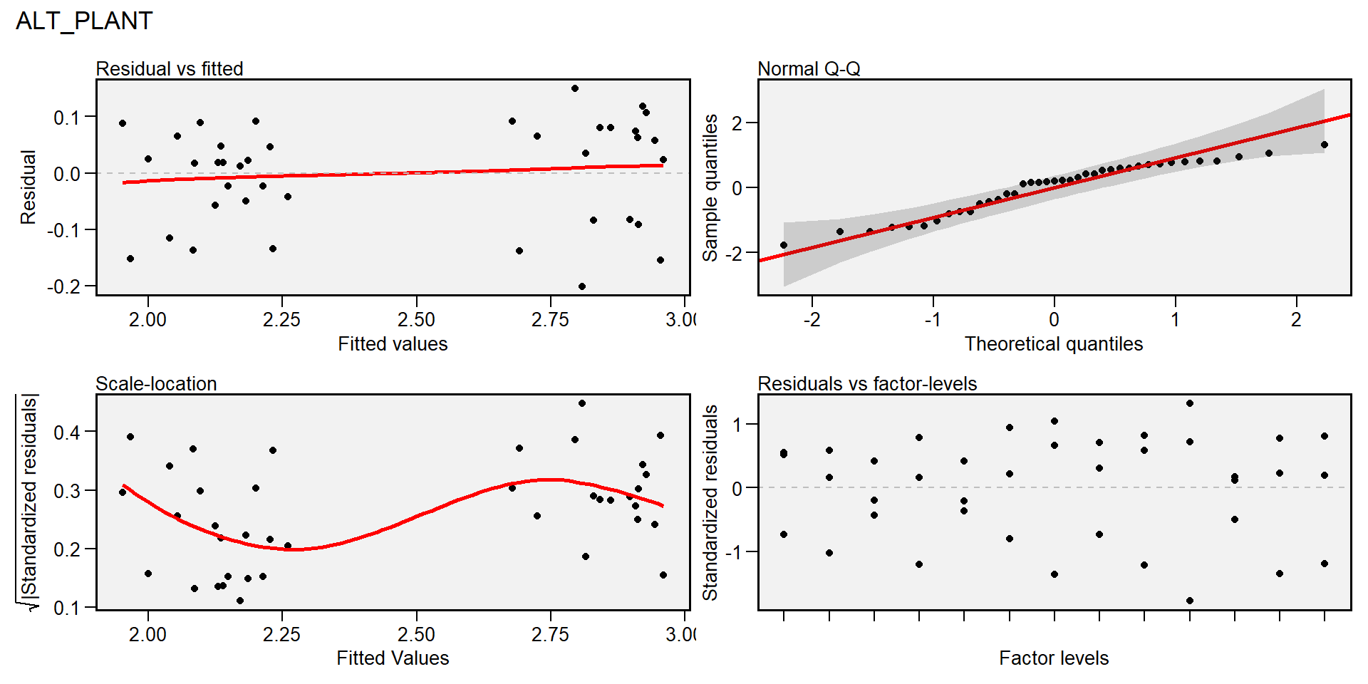
Diagnósticos do modelo
plot(gen_mod, type = "res") # padrão
## `geom_smooth()` using formula 'y ~ x'
## `geom_smooth()` using formula 'y ~ x'
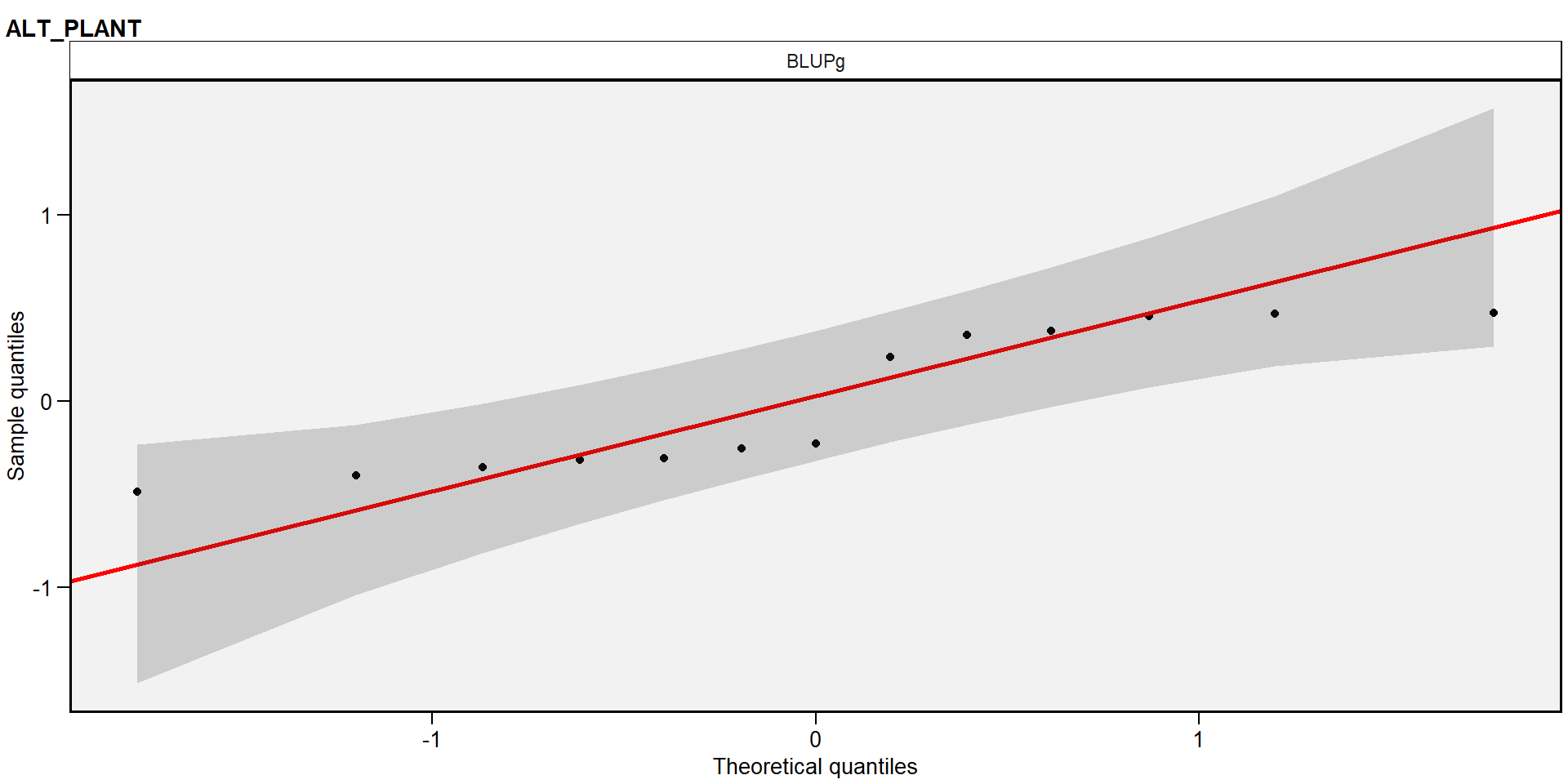
plot(gen_mod, type = "re") # padrão
Detalhes da análise
details <- gmd(gen_mod, "details")
## Class of the model: gamem
## Variable extracted: details
print_tbl(details)
| Parameters | ALT_PLANT | ALT_ESP | COMPES | DIAMES | COMP_SAB | DIAM_SAB | MGE | NFIL | MMG | NGE |
|---|---|---|---|---|---|---|---|---|---|---|
| Ngen | 13 | 13 | 13 | 13 | 13 | 13 | 13 | 13 | 13 | 13 |
| OVmean | 2.4619 | 1.3131 | 15.2333 | 48.7385 | 28.463 | 15.8874 | 168.4356 | 15.7949 | 333.8148 | 504.6513 |
| Min | 1.814 (H8 in II) | 0.752 (H8 in II) | 12.5 (H12 in III) | 44.71 (H8 in I) | 23.852 (H8 in II) | 13.28 (H12 in III) | 105.7167 (H9 in I) | 13.2 (H10 in II) | 226.5956 (H9 in III) | 354 (H12 in II) |
| Max | 3.04 (H3 in II) | 1.878 (H1 in I) | 17.94 (H6 in III) | 53.742 (H6 in III) | 33.018 (H2 in III) | 18.28 (H6 in III) | 236.1105 (H6 in III) | 18 (H13 in III) | 451.6832 (H3 in II) | 674.4 (H6 in III) |
| MinGEN | 1.9593 (H8) | 0.846 (H8) | 13.36 (H12) | 45.2607 (H8) | 24.5707 (H8) | 13.88 (H12) | 112.3297 (H9) | 13.7333 (H11) | 236.2815 (H8) | 424 (H12) |
| MaxGEN | 2.9467 (H2) | 1.7953 (H1) | 17.24 (H6) | 53.19 (H2) | 32.7087 (H2) | 17.62 (H6) | 218.8555 (H2) | 17.4667 (H2) | 415.6753 (H2) | 621.7333 (H6) |
LRT
lrt <- gmd(gen_mod, "lrt")
## Class of the model: gamem
## Variable extracted: lrt
print_tbl(lrt)
| VAR | model | npar | logLik | AIC | LRT | Df | Pr(>Chisq) |
|---|---|---|---|---|---|---|---|
| ALT_PLANT | Genotype | 4 | -22.779 | 53.557 | 49.238 | 1 | 0.000 |
| ALT_ESP | Genotype | 4 | -17.699 | 43.398 | 53.684 | 1 | 0.000 |
| COMPES | Genotype | 4 | -66.845 | 141.690 | 13.617 | 1 | 0.000 |
| DIAMES | Genotype | 4 | -91.660 | 191.320 | 24.927 | 1 | 0.000 |
| COMP_SAB | Genotype | 4 | -89.278 | 186.555 | 32.902 | 1 | 0.000 |
| DIAM_SAB | Genotype | 4 | -66.422 | 140.844 | 13.005 | 1 | 0.000 |
| MGE | Genotype | 4 | -185.644 | 379.288 | 29.849 | 1 | 0.000 |
| NFIL | Genotype | 4 | -68.094 | 144.188 | 10.145 | 1 | 0.001 |
| MMG | Genotype | 4 | -202.400 | 412.800 | 28.734 | 1 | 0.000 |
| NGE | Genotype | 4 | -202.803 | 413.607 | 6.808 | 1 | 0.009 |
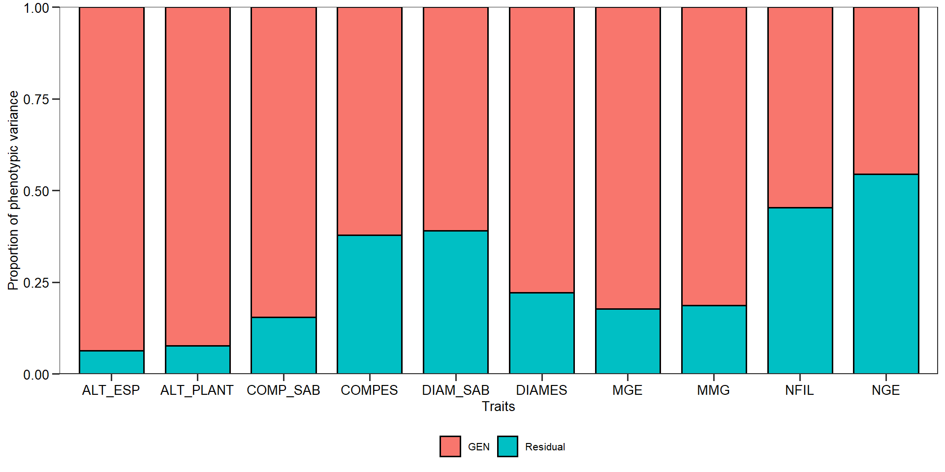
Componentes de variância
vcomp <- gmd(gen_mod, "vcomp")
## Class of the model: gamem
## Variable extracted: vcomp
print_tbl(vcomp)
| Group | ALT_PLANT | ALT_ESP | COMPES | DIAMES | COMP_SAB | DIAM_SAB | MGE | NFIL | MMG | NGE |
|---|---|---|---|---|---|---|---|---|---|---|
| GEN | 0.155 | 0.118 | 1.205 | 5.992 | 5.698 | 1.154 | 1172.429 | 1.137 | 2941.365 | 1682.787 |
| Residual | 0.013 | 0.008 | 0.734 | 1.703 | 1.043 | 0.739 | 252.595 | 0.941 | 673.583 | 2014.021 |
plot(gen_mod, type = "vcomp")
Parâmetros genéticos
genpar <- gmd(gen_mod, "genpar")
## Class of the model: gamem
## Variable extracted: genpar
print_tbl(genpar)
| Parameters | ALT_PLANT | ALT_ESP | COMPES | DIAMES | COMP_SAB | DIAM_SAB | MGE | NFIL | MMG | NGE |
|---|---|---|---|---|---|---|---|---|---|---|
| Gen_var | 0.155 | 0.118 | 1.205 | 5.992 | 5.698 | 1.154 | 1172.429 | 1.137 | 2941.365 | 1682.787 |
| Gen (%) | 92.383 | 93.700 | 62.139 | 77.867 | 84.522 | 60.954 | 82.274 | 54.722 | 81.367 | 45.520 |
| Res_var | 0.013 | 0.008 | 0.734 | 1.703 | 1.043 | 0.739 | 252.595 | 0.941 | 673.583 | 2014.021 |
| Res (%) | 7.617 | 6.300 | 37.861 | 22.133 | 15.478 | 39.046 | 17.726 | 45.278 | 18.633 | 54.480 |
| Phen_var | 0.168 | 0.126 | 1.939 | 7.695 | 6.741 | 1.894 | 1425.024 | 2.078 | 3614.948 | 3696.808 |
| H2 | 0.924 | 0.937 | 0.621 | 0.779 | 0.845 | 0.610 | 0.823 | 0.547 | 0.814 | 0.455 |
| h2mg | 0.973 | 0.978 | 0.831 | 0.913 | 0.942 | 0.824 | 0.933 | 0.784 | 0.929 | 0.715 |
| Accuracy | 0.987 | 0.989 | 0.912 | 0.956 | 0.971 | 0.908 | 0.966 | 0.885 | 0.964 | 0.845 |
| CVg | 15.983 | 26.209 | 7.205 | 5.022 | 8.386 | 6.762 | 20.329 | 6.751 | 16.247 | 8.129 |
| CVr | 4.589 | 6.796 | 5.624 | 2.678 | 3.589 | 5.412 | 9.436 | 6.141 | 7.775 | 8.893 |
| CV ratio | 3.483 | 3.857 | 1.281 | 1.876 | 2.337 | 1.249 | 2.154 | 1.099 | 2.090 | 0.914 |
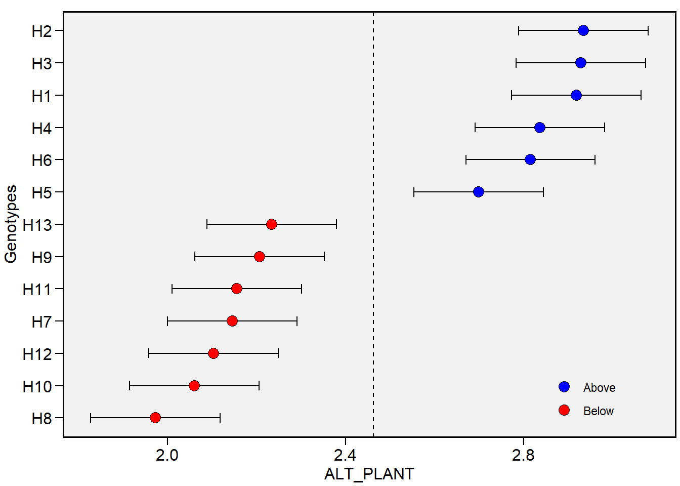
BLUPs preditos
blupg <- gmd(gen_mod, "blupg")
## Class of the model: gamem
## Variable extracted: blupg
print_tbl(blupg)
| GEN | ALT_PLANT | ALT_ESP | COMPES | DIAMES | COMP_SAB | DIAM_SAB | MGE | NFIL | MMG | NGE |
|---|---|---|---|---|---|---|---|---|---|---|
| H1 | 2.917 | 1.785 | 15.017 | 51.603 | 31.340 | 15.563 | 186.872 | 16.792 | 385.023 | 490.175 |
| H10 | 2.060 | 0.994 | 15.477 | 46.904 | 26.891 | 16.229 | 160.465 | 14.388 | 317.204 | 508.904 |
| H11 | 2.155 | 1.025 | 15.139 | 47.439 | 27.304 | 15.696 | 163.931 | 14.179 | 341.393 | 485.600 |
| H12 | 2.103 | 0.904 | 13.676 | 46.909 | 27.301 | 14.233 | 133.764 | 15.120 | 314.632 | 447.000 |
| H13 | 2.234 | 1.112 | 15.627 | 50.133 | 31.760 | 16.617 | 169.027 | 16.583 | 327.351 | 517.672 |
| H2 | 2.934 | 1.735 | 15.859 | 52.805 | 32.464 | 16.469 | 215.477 | 17.105 | 409.870 | 523.772 |
| H3 | 2.928 | 1.740 | 15.294 | 50.207 | 29.987 | 15.865 | 189.434 | 15.120 | 395.348 | 483.122 |
| H4 | 2.836 | 1.620 | 16.297 | 49.308 | 29.574 | 16.975 | 195.519 | 15.120 | 384.768 | 508.808 |
| H5 | 2.698 | 1.418 | 16.270 | 48.200 | 27.479 | 16.821 | 185.049 | 15.956 | 332.910 | 544.502 |
| H6 | 2.815 | 1.544 | 16.901 | 51.369 | 26.981 | 17.315 | 211.906 | 16.687 | 345.164 | 588.344 |
| H7 | 2.145 | 1.113 | 14.712 | 47.449 | 27.260 | 15.568 | 145.452 | 15.642 | 295.030 | 492.081 |
| H8 | 1.973 | 0.856 | 13.953 | 45.562 | 24.795 | 14.557 | 116.678 | 16.269 | 243.199 | 484.695 |
| H9 | 2.206 | 1.223 | 13.809 | 45.714 | 26.883 | 14.629 | 116.089 | 16.374 | 247.701 | 485.791 |
# plotar os BLUPS (default)
plot_blup(gen_mod)
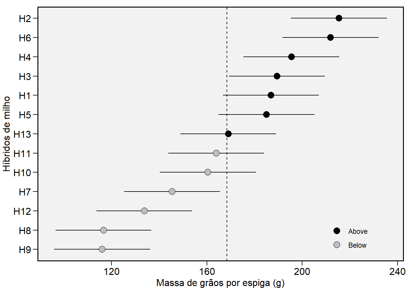
# Trait MGE
plot_blup(gen_mod,
          var = "MGE",
          height.err.bar = 0,
          col.shape = c("black", "gray"),
          x.lab = "Massa de grãos por espiga (g)",
          y.lab = "Híbridos de milho")
Modelos mistos - dentro de ambientes
df_ge <- import("http://bit.ly/df_ge", setclass = "tbl")
mod_gen_whithin <-
    gamem(df_ge,
          gen = GEN,
          rep = BLOCO,
          resp = everything(),
          by = ENV, verbose = FALSE)

gmd(mod_gen_whithin, "lrt") %>%  print_tbl()
| ENV | VAR | model | npar | logLik | AIC | LRT | Df | Pr(>Chisq) |
|---|---|---|---|---|---|---|---|---|
| A1 | ALT_PLANT | Genotype | 4 | 19.651 | -31.302 | 0.232 | 1 | 0.630 |
| A1 | ALT_ESP | Genotype | 4 | 18.480 | -28.960 | 2.134 | 1 | 0.144 |
| A1 | COMPES | Genotype | 4 | -61.532 | 131.065 | 0.000 | 1 | 1.000 |
| A1 | DIAMES | Genotype | 4 | -77.909 | 163.817 | 7.960 | 1 | 0.005 |
| A1 | COMP_SAB | Genotype | 4 | -84.379 | 176.758 | 12.568 | 1 | 0.000 |
| A1 | DIAM_SAB | Genotype | 4 | -58.807 | 125.614 | 0.103 | 1 | 0.748 |
| A1 | MGE | Genotype | 4 | -162.635 | 333.270 | 2.073 | 1 | 0.150 |
| A1 | NFIL | Genotype | 4 | -80.166 | 168.333 | 2.552 | 1 | 0.110 |
| A1 | MMG | Genotype | 4 | -186.894 | 381.789 | 3.654 | 1 | 0.056 |
| A1 | NGE | Genotype | 4 | -205.051 | 418.101 | 0.529 | 1 | 0.467 |
| A2 | ALT_PLANT | Genotype | 4 | -22.779 | 53.557 | 49.238 | 1 | 0.000 |
| A2 | ALT_ESP | Genotype | 4 | -17.699 | 43.398 | 53.684 | 1 | 0.000 |
| A2 | COMPES | Genotype | 4 | -66.845 | 141.690 | 13.617 | 1 | 0.000 |
| A2 | DIAMES | Genotype | 4 | -91.660 | 191.320 | 24.927 | 1 | 0.000 |
| A2 | COMP_SAB | Genotype | 4 | -89.278 | 186.555 | 32.902 | 1 | 0.000 |
| A2 | DIAM_SAB | Genotype | 4 | -66.422 | 140.844 | 13.005 | 1 | 0.000 |
| A2 | MGE | Genotype | 4 | -185.644 | 379.288 | 29.849 | 1 | 0.000 |
| A2 | NFIL | Genotype | 4 | -68.094 | 144.188 | 10.145 | 1 | 0.001 |
| A2 | MMG | Genotype | 4 | -202.400 | 412.800 | 28.734 | 1 | 0.000 |
| A2 | NGE | Genotype | 4 | -202.803 | 413.607 | 6.808 | 1 | 0.009 |
| A3 | ALT_PLANT | Genotype | 4 | -0.947 | 9.893 | 3.810 | 1 | 0.051 |
| A3 | ALT_ESP | Genotype | 4 | 3.562 | 0.877 | 0.561 | 1 | 0.454 |
| A3 | COMPES | Genotype | 4 | -55.480 | 118.959 | 0.073 | 1 | 0.786 |
| A3 | DIAMES | Genotype | 4 | -91.901 | 191.802 | 17.595 | 1 | 0.000 |
| A3 | COMP_SAB | Genotype | 4 | -86.207 | 180.414 | 22.367 | 1 | 0.000 |
| A3 | DIAM_SAB | Genotype | 4 | -52.489 | 112.979 | 2.449 | 1 | 0.118 |
| A3 | MGE | Genotype | 4 | -165.345 | 338.690 | 5.002 | 1 | 0.025 |
| A3 | NFIL | Genotype | 4 | -71.073 | 150.146 | 7.673 | 1 | 0.006 |
| A3 | MMG | Genotype | 4 | -190.433 | 388.866 | 6.716 | 1 | 0.010 |
| A3 | NGE | Genotype | 4 | -205.860 | 419.720 | 6.723 | 1 | 0.010 |
| A4 | ALT_PLANT | Genotype | 4 | 9.295 | -10.590 | 0.000 | 1 | 1.000 |
| A4 | ALT_ESP | Genotype | 4 | 13.658 | -19.316 | 0.000 | 1 | 1.000 |
| A4 | COMPES | Genotype | 4 | -65.282 | 138.564 | 6.803 | 1 | 0.009 |
| A4 | DIAMES | Genotype | 4 | -83.220 | 174.441 | 0.235 | 1 | 0.628 |
| A4 | COMP_SAB | Genotype | 4 | -76.511 | 161.022 | 4.359 | 1 | 0.037 |
| A4 | DIAM_SAB | Genotype | 4 | -62.685 | 133.371 | 3.074 | 1 | 0.080 |
| A4 | MGE | Genotype | 4 | -174.257 | 356.514 | 0.095 | 1 | 0.758 |
| A4 | NFIL | Genotype | 4 | -65.683 | 139.366 | 1.401 | 1 | 0.237 |
| A4 | MMG | Genotype | 4 | -183.409 | 374.818 | 1.755 | 1 | 0.185 |
| A4 | NGE | Genotype | 4 | -210.085 | 428.170 | 0.966 | 1 | 0.326 |
gmd(mod_gen_whithin, "vcomp") %>% print_tbl()
| ENV | Group | ALT_PLANT | ALT_ESP | COMPES | DIAMES | COMP_SAB | DIAM_SAB | MGE | NFIL | MMG | NGE |
|---|---|---|---|---|---|---|---|---|---|---|---|
| A1 | GEN | 0.001 | 0.004 | 0.000 | 1.756 | 3.085 | 0.068 | 100.060 | 1.139 | 512.906 | 524.620 |
| A1 | Residual | 0.015 | 0.013 | 1.443 | 1.828 | 2.050 | 1.173 | 296.826 | 2.925 | 1014.606 | 3663.805 |
| A2 | GEN | 0.155 | 0.118 | 1.205 | 5.992 | 5.698 | 1.154 | 1172.429 | 1.137 | 2941.365 | 1682.787 |
| A2 | Residual | 0.013 | 0.008 | 0.734 | 1.703 | 1.043 | 0.739 | 252.595 | 0.941 | 673.583 | 2014.021 |
| A3 | GEN | 0.017 | 0.005 | 0.047 | 5.369 | 4.269 | 0.240 | 180.972 | 1.181 | 840.939 | 1982.321 |
| A3 | Residual | 0.033 | 0.034 | 0.984 | 2.430 | 1.415 | 0.634 | 280.409 | 1.271 | 1018.430 | 2398.781 |
| A4 | GEN | 0.000 | 0.000 | 0.809 | 0.398 | 1.216 | 0.474 | 39.561 | 0.375 | 291.452 | 944.826 |
| A4 | Residual | 0.028 | 0.022 | 0.969 | 4.417 | 2.101 | 1.065 | 717.405 | 1.442 | 967.158 | 4595.334 |