Modelos biométricos
library(metan)
## Registered S3 method overwritten by 'GGally':
##   method from
##   +.gg   ggplot2
## |=========================================================|
## | Multi-Environment Trial Analysis (metan) v1.15.0        |
## | Author: Tiago Olivoto                                   |
## | Type 'citation('metan')' to know how to cite metan      |
## | Type 'vignette('metan_start')' for a short tutorial     |
## | Visit 'https://bit.ly/pkgmetan' for a complete tutorial |
## |=========================================================|
library(rio)
# gerar tabelas html
print_tbl <- function(table, digits = 3, ...){
  knitr::kable(table, booktabs = TRUE, digits = digits, ...)
}
df_ge <- import("http://bit.ly/df_ge", setclass = "tbl")
Correlação linear
A função corr_coef() pode ser usada para calcular o coeficiente de correlação de Pearson com valores de p. Um mapa de calor de correlação pode ser criado com a função plot().
# Todas as variáveis numéricas
ccoef <- corr_coef(df_ge)
plot(ccoef)
## Warning: Removed 5 rows containing missing values (geom_text).

Podemos usar uma função auxiliar de seleção para selecionar variáveis. Aqui, selecionaremos variáveis que começam com “C” ** OU ** termina com “D” usando union_var ().
ccoef2 <- corr_coef(df_ge, contains("A"))
plot(ccoef2, dígitos = 2)

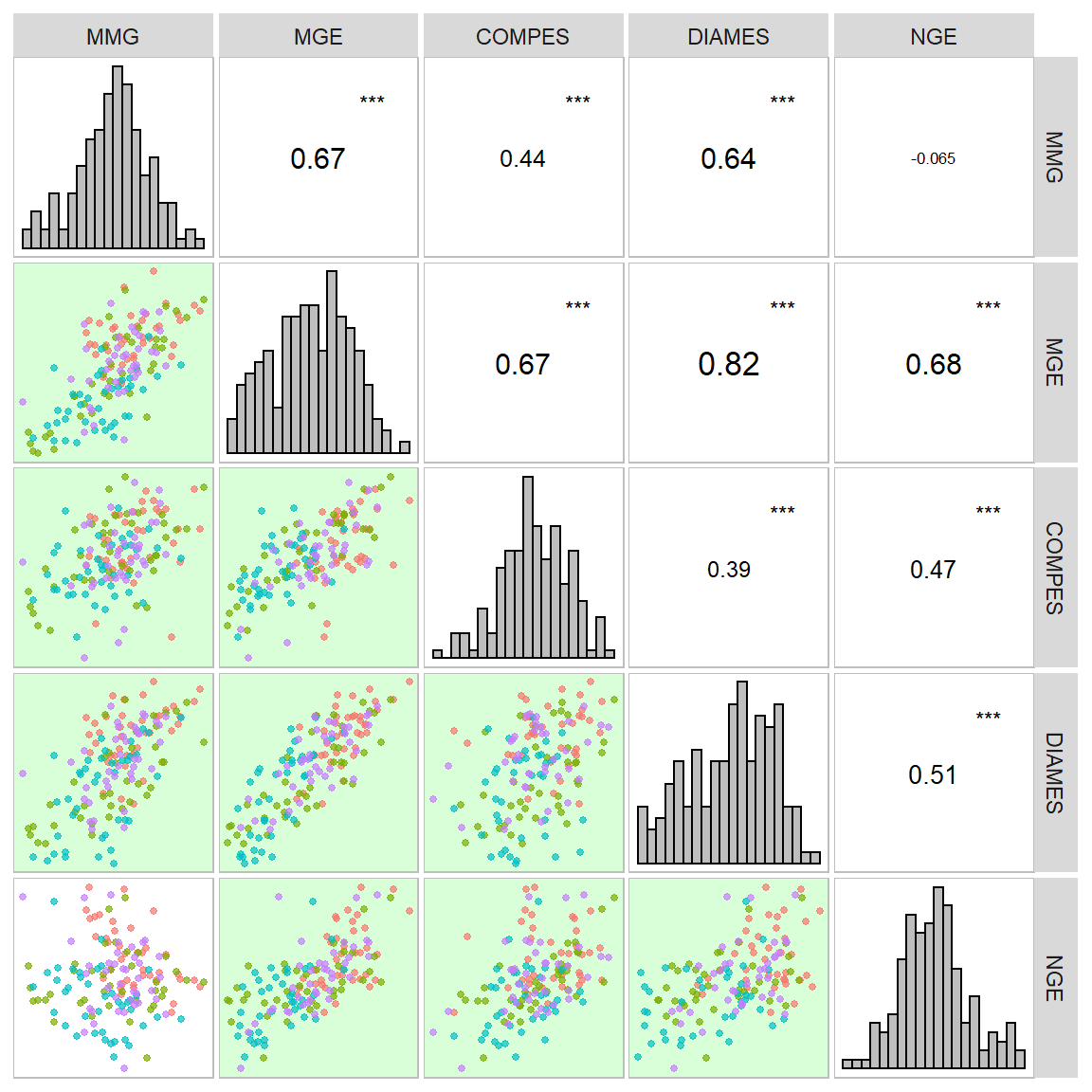
A função corr_plot() pode ser usada para visualizar (graficamente e numericamente) uma matriz de correlação. Os gráficos de dispersão em pares são produzidos e podem ser mostrados na diagonal superior ou inferior, o que pode ser visto como uma versão mais agradável e personalizável baseada em ggplot2 da função R de base de pairs().
a <- corr_plot(df_ge, MMG, MGE, COMPES, DIAMES, NGE)


corr_plot(df_ge, MMG, MGE, COMPES, DIAMES, NGE,
          lower = NULL,
          upper = "corr")

corr_plot(df_ge, MMG, MGE, COMPES, DIAMES, NGE,
          shape.point = 19,
          size.point = 2,
          alpha.point = 0.5,
          alpha.diag = 0,
          pan.spacing = 0,
          diag.type = "boxplot",
          col.sign = "gray",
          alpha.sign = 0.3,
          axis.labels = TRUE)

corr_plot(df_ge, MMG, MGE, COMPES, DIAMES, NGE,
          prob = 0.01,
          shape.point = 21,
          col.point = "black",
          fill.point = "orange",
          size.point = 2,
          alpha.point = 0.6,
          maxsize = 4,
          minsize = 2,
          smooth = TRUE,
          size.smooth = 1,
          col.smooth = "black",
          col.sign = "cyan",
          col.up.panel = "black",
          col.lw.panel = "black",
          col.dia.panel = "black",
          pan.spacing = 0,
          lab.position = "tl")
Também é possível usar uma variável categórica dos dados para mapear o gráfico de dispersão por cores.
corr_plot(df_ge, MMG, MGE, COMPES, DIAMES, NGE, col.by = ENV)
Matrizes de correlação/covariância
A função covcor_design() pode ser usada para calcular matrizes de correlação genéticas, fenotípicas e residuais de correlação por meio da Análise de Variância (ANOVA) usando um delineamento de bloco completo ao acaso (DBC) ou delineamento inteiramente ao acaso (DIC).
As correlações fenotípicas (\(r_p\)), genotípicas (\(r_g\)) e residuais (\(r_r\)) são calculadas da seguinte forma:
$$
r ^ p_ {xy} = \frac {cov ^ p_ {xy}} {\sqrt {var ^ p_ {x} var ^ p_ {y}}} \
r ^ g_ {xy} = \frac {cov ^ g_ {xy}} {\sqrt {var ^ g_ {x} var ^ g_ {y}}} \
r ^ r_ {xy} = \frac {cov ^ r_ {xy}} {\sqrt {var ^ r_ {x} var ^ r_ {y}}}
$$
Usando os quadrados médios (MS) do método ANOVA, as variâncias (var) e as covariâncias (cov) são calculadas da seguinte forma:
$$
cov ^ p_ {xy} = [(MST_ {x + y} - MST_x - MST_y) / 2] / r \
var ^ p_x = MST_x / r \
var ^ p_y = MST_y / r \
cov ^ r_ {xy} = (MSR_ {x + y} - MSR_x - MSR_y) / 2 \
var ^ r_x = MSR_x \
var ^ r_y = MSR_y \
cov ^ g_ {xy} = [(cov ^ p_ {xy} \times r) - cov ^ r_ {xy}] / r \
var ^ g_x = (MST_x - MSE_x) / r \
var ^ g_y = (MST_x - MSE_y) / r \
$$
onde \(MST\) é o quadrado médio para tratamento, \(MSR\) é o quadrado médio para resíduos e \(r\) é o número de repetições. A função covcor_design() retorna uma lista com as matrize. Matrizes específicas podem ser retornadas usando o argumento type, conforme mostrado abaixo.
df_g <- import("http://bit.ly/df_g", setclass = "tbl")
correl <- covcor_design(df_g,
                        gen = GEN,
                        rep = BLOCO,
                        resp = c(MMG, MGE, COMPES, DIAMES, NGE))
Correlações
# genéticas
print_tbl(correl$geno_cor)
| MMG | MGE | COMPES | DIAMES | NGE | |
|---|---|---|---|---|---|
| MMG | 1.000 | 0.927 | 0.671 | 0.906 | 0.368 |
| MGE | 0.927 | 1.000 | 0.918 | 0.933 | 0.692 |
| COMPES | 0.671 | 0.918 | 1.000 | 0.752 | 0.992 |
| DIAMES | 0.906 | 0.933 | 0.752 | 1.000 | 0.561 |
| NGE | 0.368 | 0.692 | 0.992 | 0.561 | 1.000 |
# fenotípicas
print_tbl(correl$phen_cor)
| MMG | MGE | COMPES | DIAMES | NGE | |
|---|---|---|---|---|---|
| MMG | 1.000 | 0.893 | 0.628 | 0.852 | 0.241 |
| MGE | 0.893 | 1.000 | 0.883 | 0.897 | 0.651 |
| COMPES | 0.628 | 0.883 | 1.000 | 0.661 | 0.854 |
| DIAMES | 0.852 | 0.897 | 0.661 | 1.000 | 0.496 |
| NGE | 0.241 | 0.651 | 0.854 | 0.496 | 1.000 |
# residuais
print_tbl(correl$resi_cor)
| MMG | MGE | COMPES | DIAMES | NGE | |
|---|---|---|---|---|---|
| MMG | 1.000 | 0.431 | 0.348 | 0.223 | -0.417 |
| MGE | 0.431 | 1.000 | 0.704 | 0.466 | 0.624 |
| COMPES | 0.348 | 0.704 | 1.000 | 0.050 | 0.408 |
| DIAMES | 0.223 | 0.466 | 0.050 | 1.000 | 0.275 |
| NGE | -0.417 | 0.624 | 0.408 | 0.275 | 1.000 |
Covariâncias
# genéticas
print_tbl(correl$geno_cov)
| MMG | MGE | COMPES | DIAMES | NGE | |
|---|---|---|---|---|---|
| MMG | 2941.365 | 1721.242 | 39.930 | 120.289 | 819.553 |
| MGE | 1721.242 | 1172.429 | 34.496 | 78.218 | 971.370 |
| COMPES | 39.930 | 34.496 | 1.205 | 2.020 | 44.672 |
| DIAMES | 120.289 | 78.218 | 2.020 | 5.992 | 56.286 |
| NGE | 819.553 | 971.370 | 44.672 | 56.286 | 1682.787 |
# fenotípicas
print_tbl(correl$phen_cov)
| MMG | MGE | COMPES | DIAMES | NGE | |
|---|---|---|---|---|---|
| MMG | 3165.893 | 1780.539 | 42.506 | 122.810 | 657.574 |
| MGE | 1780.539 | 1256.627 | 37.692 | 81.442 | 1119.668 |
| COMPES | 42.506 | 37.692 | 1.449 | 2.038 | 49.899 |
| DIAMES | 122.810 | 81.442 | 2.038 | 6.560 | 61.649 |
| NGE | 657.574 | 1119.668 | 49.899 | 61.649 | 2354.128 |
# residuais
print_tbl(correl$resi_cov)
| MMG | MGE | COMPES | DIAMES | NGE | |
|---|---|---|---|---|---|
| MMG | 673.583 | 177.892 | 7.730 | 7.564 | -485.939 |
| MGE | 177.892 | 252.595 | 9.588 | 9.672 | 444.893 |
| COMPES | 7.730 | 9.588 | 0.734 | 0.056 | 15.681 |
| DIAMES | 7.564 | 9.672 | 0.056 | 1.703 | 16.090 |
| NGE | -485.939 | 444.893 | 15.681 | 16.090 | 2014.021 |
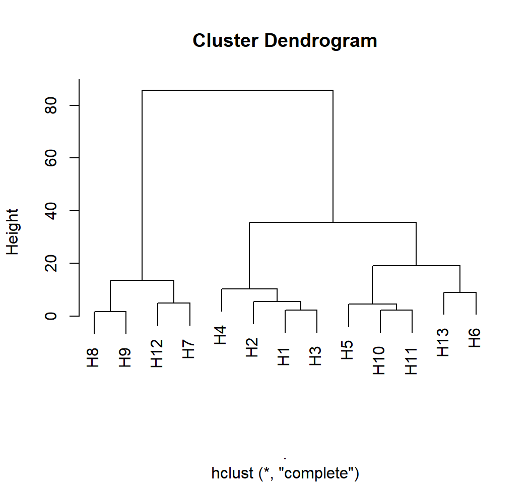
Distância de Mahalanobis
A matriz de covariância residual e as médias podem ser usados na função mahala() para calcular a distância de Mahalanobis.
D2 <- mahala(.means = correl$means, covar = correl$resi_cov, inverted = FALSE)
print_tbl(D2)
| H1 | H10 | H11 | H12 | H13 | H2 | H3 | H4 | H5 | H6 | H7 | H8 | H9 | |
|---|---|---|---|---|---|---|---|---|---|---|---|---|---|
| H1 | 0.000 | 22.376 | 14.474 | 23.648 | 12.483 | 3.844 | 2.334 | 7.508 | 17.464 | 14.837 | 26.980 | 59.690 | 51.562 |
| H10 | 22.376 | 0.000 | 2.334 | 8.772 | 9.100 | 35.607 | 18.127 | 10.696 | 2.903 | 18.311 | 5.290 | 18.563 | 13.522 |
| H11 | 14.474 | 2.334 | 0.000 | 5.474 | 10.975 | 25.937 | 9.655 | 6.592 | 4.653 | 19.124 | 6.482 | 23.686 | 19.195 |
| H12 | 23.648 | 8.772 | 5.474 | 0.000 | 18.393 | 42.726 | 20.782 | 22.110 | 17.671 | 37.538 | 4.956 | 13.675 | 10.465 |
| H13 | 12.483 | 9.100 | 10.975 | 18.393 | 0.000 | 23.219 | 16.462 | 11.848 | 7.893 | 9.072 | 10.616 | 30.521 | 24.450 |
| H2 | 3.844 | 35.607 | 25.937 | 42.726 | 23.219 | 0.000 | 5.541 | 10.274 | 24.275 | 14.521 | 44.357 | 85.575 | 77.169 |
| H3 | 2.334 | 18.127 | 9.655 | 20.782 | 16.462 | 5.541 | 0.000 | 3.420 | 13.807 | 16.940 | 26.131 | 58.552 | 50.893 |
| H4 | 7.508 | 10.696 | 6.592 | 22.110 | 11.848 | 10.274 | 3.420 | 0.000 | 5.399 | 9.827 | 21.315 | 51.358 | 44.707 |
| H5 | 17.464 | 2.903 | 4.653 | 17.671 | 7.893 | 24.275 | 13.807 | 5.399 | 0.000 | 7.806 | 11.084 | 31.217 | 25.982 |
| H6 | 14.837 | 18.311 | 19.124 | 37.538 | 9.072 | 14.521 | 16.940 | 9.827 | 7.806 | 0.000 | 25.371 | 54.420 | 49.052 |
| H7 | 26.980 | 5.290 | 6.482 | 4.956 | 10.616 | 44.357 | 26.131 | 21.315 | 11.084 | 25.371 | 0.000 | 6.956 | 6.100 |
| H8 | 59.690 | 18.563 | 23.686 | 13.675 | 30.521 | 85.575 | 58.552 | 51.358 | 31.217 | 54.420 | 6.956 | 0.000 | 1.796 |
| H9 | 51.562 | 13.522 | 19.195 | 10.465 | 24.450 | 77.169 | 50.893 | 44.707 | 25.982 | 49.052 | 6.100 | 1.796 | 0.000 |
D2 %>%
  as.dist() %>%
  hclust() %>%
  plot()
Diagnóstico de colinearidade
Os códigos a seguir calculam um diagnóstico de colinearidade completo de uma matriz de correlação de características do preditor. Vários indicadores, como fator de inflação de variância, número de condição e determinante da matriz são considerados1
colin <- colindiag(df_ge)
print(colin)
## The multicollinearity in the matrix should be investigated.
## CN = 607.708
## Largest VIF = 55.4696961923099
## Matrix determinant: 1.7e-06
## Largest correlation: ALT_PLANT x ALT_ESP = 0.932
## Smallest correlation: COMPES x NFIL = -0.014
## Number of VIFs > 10: 4
## Number of correlations with r >= |0.8|: 3
## Variables with largest weight in the last eigenvalues:
## MGE > NGE > MMG > ALT_ESP > ALT_PLANT > DIAMES > DIAM_SAB > NFIL > COMPES > COMP_SAB

print_tbl(colin$evalevet)
| Eigenvalues | ALT_PLANT | ALT_ESP | COMPES | DIAMES | COMP_SAB | DIAM_SAB | MGE | NFIL | MMG | NGE |
|---|---|---|---|---|---|---|---|---|---|---|
| 5.275 | -0.358 | -0.346 | -0.297 | -0.382 | -0.263 | -0.283 | -0.416 | -0.178 | -0.306 | -0.265 |
| 1.669 | 0.106 | 0.066 | -0.311 | 0.137 | -0.119 | -0.344 | 0.012 | 0.634 | -0.398 | 0.420 |
| 1.448 | -0.163 | -0.219 | 0.464 | -0.201 | -0.389 | 0.452 | 0.085 | -0.010 | -0.335 | 0.440 |
| 0.914 | 0.498 | 0.487 | -0.049 | -0.260 | -0.568 | -0.163 | 0.035 | -0.306 | 0.000 | 0.011 |
| 0.294 | -0.155 | -0.419 | -0.208 | 0.301 | -0.474 | -0.194 | 0.421 | -0.105 | 0.447 | 0.128 |
| 0.179 | -0.175 | 0.111 | -0.190 | 0.012 | 0.370 | -0.215 | 0.221 | -0.615 | -0.249 | 0.498 |
| 0.092 | 0.194 | -0.054 | -0.504 | 0.465 | -0.120 | 0.574 | -0.239 | -0.197 | -0.220 | -0.033 |
| 0.073 | -0.216 | 0.201 | 0.457 | 0.644 | -0.197 | -0.317 | -0.250 | -0.151 | -0.216 | -0.135 |
| 0.047 | 0.668 | -0.598 | 0.237 | 0.064 | 0.164 | -0.237 | -0.120 | -0.147 | -0.124 | 0.042 |
| 0.009 | 0.033 | -0.038 | -0.009 | 0.024 | 0.006 | 0.019 | 0.677 | 0.011 | -0.514 | -0.523 |
Diagnóstico para cada nível do fator ENV
colin2 <- colindiag(df_ge, by = ENV)
print(colin2)
## # A tibble: 4 x 2
##   ENV   data
##   <chr> <list>
## 1 A1    <colindig>
## 2 A2    <colindig>
## 3 A3    <colindig>
## 4 A4    <colindig>
Análise de trilha
Neste exemplo, a variável massa de grãos por espiga (MGE) será utilziada como resposta e todas as outras como explicativa
pcoeff <- path_coeff(df_ge, resp = MGE)
## Weak multicollinearity.
## Condition Number = 97.581
## You will probably have path coefficients close to being unbiased.
print(pcoeff)
## ----------------------------------------------------------------------------------------------
## Correlation matrix between the predictor traits
## ----------------------------------------------------------------------------------------------
##           ALT_PLANT ALT_ESP   COMPES DIAMES COMP_SAB DIAM_SAB     NFIL      MMG
## ALT_PLANT    1.0000  0.9318  0.38020 0.6613  0.32516  0.31539  0.32861  0.56854
## ALT_ESP      0.9318  1.0000  0.36265 0.6303  0.39719  0.28051  0.26481  0.56236
## COMPES       0.3802  0.3627  1.00000 0.3851  0.25541  0.91187 -0.01387  0.44210
## DIAMES       0.6613  0.6303  0.38515 1.0000  0.69746  0.38971  0.55253  0.64199
## COMP_SAB     0.3252  0.3972  0.25541 0.6975  1.00000  0.30036  0.26194  0.61870
## DIAM_SAB     0.3154  0.2805  0.91187 0.3897  0.30036  1.00000 -0.03585  0.44332
## NFIL         0.3286  0.2648 -0.01387 0.5525  0.26194 -0.03585  1.00000 -0.10876
## MMG          0.5685  0.5624  0.44210 0.6420  0.61870  0.44332 -0.10876  1.00000
## NGE          0.4584  0.3881  0.46570 0.5051  0.04894  0.41562  0.62609 -0.06516
##                NGE
## ALT_PLANT  0.45838
## ALT_ESP    0.38812
## COMPES     0.46570
## DIAMES     0.50508
## COMP_SAB   0.04894
## DIAM_SAB   0.41562
## NFIL       0.62609
## MMG       -0.06516
## NGE        1.00000
## ----------------------------------------------------------------------------------------------
## Vector of correlations between dependent and each predictor
## ----------------------------------------------------------------------------------------------
##     ALT_PLANT   ALT_ESP    COMPES    DIAMES COMP_SAB  DIAM_SAB      NFIL
## MGE 0.7534439 0.7029469 0.6685601 0.8241426 0.470931 0.6259806 0.3621447
##           MMG       NGE
## MGE 0.6730371 0.6810756
## ----------------------------------------------------------------------------------------------
## Multicollinearity diagnosis and goodness-of-fit
## ----------------------------------------------------------------------------------------------
## Condition number:  97.5813
## Determinant:       9.241e-05
## R-square:          0.982
## Residual:          0.1343
## Response:          MGE
## Predictors:        ALT_PLANT ALT_ESP COMPES DIAMES COMP_SAB DIAM_SAB NFIL MMG NGE
## ----------------------------------------------------------------------------------------------
## Variance inflation factors
## ----------------------------------------------------------------------------------------------
## # A tibble: 9 x 2
##   VAR          VIF
##   <chr>      <dbl>
## 1 ALT_PLANT 11.30
## 2 ALT_ESP    9.302
## 3 COMPES     7.331
## 4 DIAMES     8.636
## 5 COMP_SAB   3.270
## 6 DIAM_SAB   6.814
## 7 NFIL       3.676
## 8 MMG        6.965
## 9 NGE        5.396
## ----------------------------------------------------------------------------------------------
## Eigenvalues and eigenvectors
## ----------------------------------------------------------------------------------------------
## # A tibble: 9 x 10
##   Eigenvalues ALT_PLANT  ALT_ESP   COMPES  DIAMES COMP_SAB DIAM_SAB     NFIL
##         <dbl>     <dbl>    <dbl>    <dbl>   <dbl>    <dbl>    <dbl>    <dbl>
## 1     4.382    -0.3957  -0.3860  -0.3207  -0.4210 -0.3025  -0.3069  -0.1968
## 2     1.669    -0.1105  -0.07139  0.3116  -0.1422  0.1131   0.3450  -0.6359
## 3     1.436    -0.1416  -0.1977   0.4834  -0.1783 -0.3687   0.4719   0.01084
## 4     0.9130    0.5057   0.4952  -0.03763 -0.2558 -0.5642  -0.1520  -0.3006
## 5     0.2429    0.03453  0.3984   0.1010  -0.4234  0.5823   0.05879 -0.06332
## 6     0.1638   -0.1483   0.01160 -0.2195   0.2790  0.1830  -0.1836  -0.6531
## 7     0.08619  -0.2376   0.08451  0.6328  -0.1318  0.03175 -0.6776   0.06203
## 8     0.06259  -0.2610   0.3031   0.2035   0.6326 -0.2275  -0.01768 -0.09131
## 9     0.04490   0.6385  -0.5511   0.2544   0.1748  0.1271  -0.2106  -0.1540
## # ... with 2 more variables: MMG <dbl>, NGE <dbl>
## ----------------------------------------------------------------------------------------------
## Variables with the largest weight in the eigenvalue of smallest magnitude
## ----------------------------------------------------------------------------------------------
## ALT_PLANT > ALT_ESP > MMG > COMPES > DIAM_SAB > DIAMES > NFIL > NGE > COMP_SAB
## ----------------------------------------------------------------------------------------------
## Direct (diagonal) and indirect (off-diagonal) effects
## ----------------------------------------------------------------------------------------------
##              ALT_PLANT    ALT_ESP        COMPES      DIAMES      COMP_SAB
## ALT_PLANT -0.013315310 0.04002135  0.0138641226 0.015196362 -0.0047188442
## ALT_ESP   -0.012407581 0.04294928  0.0132244307 0.014482662 -0.0057641364
## COMPES    -0.005062428 0.01557572  0.0364657233 0.008850255 -0.0037065040
## DIAMES    -0.008805612 0.02706905  0.0140445955 0.022979012 -0.0101216939
## COMP_SAB  -0.004329670 0.01705918  0.0093135921 0.016027009 -0.0145121611
## DIAM_SAB  -0.004199528 0.01204778  0.0332518264 0.008955216 -0.0043589255
## NFIL      -0.004375497 0.01137319 -0.0005059176 0.012696697 -0.0038012563
## MMG       -0.007570266 0.02415282  0.0161215357 0.014752226 -0.0089786759
## NGE       -0.006103472 0.01666954  0.0169820638 0.011606259 -0.0007102577
##                DIAM_SAB          NFIL        MMG         NGE    linear
## ALT_PLANT -0.0067498812 -0.0082032241  0.3909975  0.32635179 0.7534439
## ALT_ESP   -0.0060034106 -0.0066105076  0.3867462  0.27632993 0.7029469
## COMPES    -0.0195154051  0.0003463406  0.3040435  0.33156290 0.6685601
## DIAMES    -0.0083404905 -0.0137932898  0.4415098  0.35960124 0.8241426
## COMP_SAB  -0.0064282721 -0.0065388826  0.4254949  0.03484530 0.4709310
## DIAM_SAB  -0.0214016323  0.0008949437  0.3048852  0.29590577 0.6259806
## NFIL       0.0007672451 -0.0249636726 -0.0747987  0.44575261 0.3621447
## MMG       -0.0094878766  0.0027151156  0.6877240 -0.04639172 0.6730371
## NGE       -0.0088948788 -0.0156293919 -0.0448120  0.71196770 0.6810756
## ----------------------------------------------------------------------------------------------
Para declarar características preditoras, use o argumento pred
pcoeff2 <-
  path_coeff(df_ge,
             resp = MGE,
             pred = c(MMG, COMPES, DIAMES, NGE))
## Weak multicollinearity.
## Condition Number = 24.907
## You will probably have path coefficients close to being unbiased.
print(pcoeff2)
## ----------------------------------------------------------------------------------------------
## Correlation matrix between the predictor traits
## ----------------------------------------------------------------------------------------------
##             MMG COMPES DIAMES      NGE
## MMG     1.00000 0.4421 0.6420 -0.06516
## COMPES  0.44210 1.0000 0.3851  0.46570
## DIAMES  0.64199 0.3851 1.0000  0.50508
## NGE    -0.06516 0.4657 0.5051  1.00000
## ----------------------------------------------------------------------------------------------
## Vector of correlations between dependent and each predictor
## ----------------------------------------------------------------------------------------------
##           MMG    COMPES    DIAMES       NGE
## MGE 0.6730371 0.6685601 0.8241426 0.6810756
## ----------------------------------------------------------------------------------------------
## Multicollinearity diagnosis and goodness-of-fit
## ----------------------------------------------------------------------------------------------
## Condition number:  24.9068
## Determinant:       0.1311275
## R-square:          0.981
## Residual:          0.1379
## Response:          MGE
## Predictors:        MMG COMPES DIAMES NGE
## ----------------------------------------------------------------------------------------------
## Variance inflation factors
## ----------------------------------------------------------------------------------------------
## # A tibble: 4 x 2
##   VAR      VIF
##   <chr>  <dbl>
## 1 MMG    4.277
## 2 COMPES 2.183
## 3 DIAMES 4.245
## 4 NGE    3.529
## ----------------------------------------------------------------------------------------------
## Eigenvalues and eigenvectors
## ----------------------------------------------------------------------------------------------
## # A tibble: 4 x 5
##   Eigenvalues      MMG  COMPES   DIAMES     NGE
##         <dbl>    <dbl>   <dbl>    <dbl>   <dbl>
## 1     2.217   -0.4726  -0.5146 -0.5837  -0.4137
## 2     1.077   -0.6640   0.1302 -0.09487  0.7302
## 3     0.6170  -0.02383 -0.7914  0.5790   0.1947
## 4     0.08902  0.5790  -0.3032 -0.5613   0.5076
## ----------------------------------------------------------------------------------------------
## Variables with the largest weight in the eigenvalue of smallest magnitude
## ----------------------------------------------------------------------------------------------
## MMG > DIAMES > NGE > COMPES
## ----------------------------------------------------------------------------------------------
## Direct (diagonal) and indirect (off-diagonal) effects
## ----------------------------------------------------------------------------------------------
##               MMG      COMPES       DIAMES         NGE    linear
## MMG     0.7207458 0.007125379 -0.007499726 -0.04733433 0.6730371
## COMPES  0.3186425 0.016117081 -0.004499286  0.33829981 0.6685601
## DIAMES  0.4627094 0.006207415 -0.011682054  0.36690786 0.8241426
## NGE    -0.0469637 0.007505714 -0.005900382  0.72643393 0.6810756
## ----------------------------------------------------------------------------------------------
Para selecionando um conjunto de preditores com multicolinearidade mínima use o argumento brutstep.
pcoeff3 <-
  path_coeff(df_ge,
             resp = MGE,
             brutstep = TRUE)
## --------------------------------------------------------------------------
## The algorithm has selected a set of 8 predictors with largest VIF = 8.634.
## Selected predictors: ALT_ESP COMP_SAB NFIL NGE MMG DIAM_SAB COMPES DIAMES
## A forward stepwise-based selection procedure will fit 6 models.
## --------------------------------------------------------------------------
## Adjusting the model 1 with 7 predictors (16.67% concluded)
## Adjusting the model 2 with 6 predictors (33.33% concluded)
## Adjusting the model 3 with 5 predictors (50% concluded)
## Adjusting the model 4 with 4 predictors (66.67% concluded)
## Adjusting the model 5 with 3 predictors (83.33% concluded)
## Adjusting the model 6 with 2 predictors (100% concluded)
## Done!
## --------------------------------------------------------------------------
## Summary of the adjusted models
## --------------------------------------------------------------------------
##    Model  AIC Numpred    CN Determinant    R2 Residual maxVIF
##  MODEL_1  923       7 51.94     0.00291 0.982    0.135   7.21
##  MODEL_2  921       6 42.05     0.01919 0.982    0.135   6.61
##  MODEL_3  921       5 34.25     0.06367 0.982    0.136   5.15
##  MODEL_4  924       4 24.91     0.13113 0.981    0.138   4.28
##  MODEL_5 1234       3  4.00     0.56087 0.860    0.375   1.52
##  MODEL_6 1267       2  2.25     0.85166 0.824    0.420   1.17
## --------------------------------------------------------------------------
print(pcoeff3$Models$Model_4)
## ----------------------------------------------------------------------------------------------
## Correlation matrix between the predictor traits
## ----------------------------------------------------------------------------------------------
##        DIAMES COMPES      NGE      MMG
## DIAMES 1.0000 0.3851  0.50508  0.64199
## COMPES 0.3851 1.0000  0.46570  0.44210
## NGE    0.5051 0.4657  1.00000 -0.06516
## MMG    0.6420 0.4421 -0.06516  1.00000
## ----------------------------------------------------------------------------------------------
## Vector of correlations between dependent and each predictor
## ----------------------------------------------------------------------------------------------
##        DIAMES    COMPES       NGE       MMG
## MGE 0.8241426 0.6685601 0.6810756 0.6730371
## ----------------------------------------------------------------------------------------------
## Multicollinearity diagnosis and goodness-of-fit
## ----------------------------------------------------------------------------------------------
## Condition number:  24.9068
## Determinant:       0.1311275
## R-square:          0.981
## Residual:          0.1379
## Response:          MGE
## Predictors:        DIAMES COMPES NGE MMG
## ----------------------------------------------------------------------------------------------
## Variance inflation factors
## ----------------------------------------------------------------------------------------------
##             VIF
## DIAMES 4.244679
## COMPES 2.182940
## NGE    3.528542
## MMG    4.277252
## ----------------------------------------------------------------------------------------------
## Eigenvalues and eigenvectors
## ----------------------------------------------------------------------------------------------
##   Eigenvalues     DIAMES      COMPES         NGE        MMG
## 1  2.21731979 -0.5836962  0.09487169  0.57897124  0.5613292
## 2  1.07668055 -0.5145820 -0.13022977 -0.79140140  0.3031986
## 3  0.61697486 -0.4137466 -0.73021132  0.19470094 -0.5076383
## 4  0.08902479 -0.4725652  0.66395105 -0.02382582 -0.5790367
## ----------------------------------------------------------------------------------------------
## Variables with the largest weight in the eigenvalue of smallest magnitude
## ----------------------------------------------------------------------------------------------
## COMPES > MMG > DIAMES > NGE
## ----------------------------------------------------------------------------------------------
## Direct (diagonal) and indirect (off-diagonal) effects
## ----------------------------------------------------------------------------------------------
##              DIAMES      COMPES         NGE        MMG    linear
## DIAMES -0.011682054 0.006207415  0.36690786  0.4627094 0.8241426
## COMPES -0.004499286 0.016117081  0.33829981  0.3186425 0.6685601
## NGE    -0.005900382 0.007505714  0.72643393 -0.0469637 0.6810756
## MMG    -0.007499726 0.007125379 -0.04733433  0.7207458 0.6730371
## ----------------------------------------------------------------------------------------------
Também é possível calcular uma análise para cada nível de um determinado fator
pcoeff4 <-
path_coeff(df_ge,
resp = MGE,
pred = c(MMG, COMPES, DIAMES, NGE),
by = ENV)
## Weak multicollinearity.
## Condition Number = 11.26
## You will probably have path coefficients close to being unbiased.
## Weak multicollinearity.
## Condition Number = 48.08
## You will probably have path coefficients close to being unbiased.
## Weak multicollinearity.
## Condition Number = 20.594
## You will probably have path coefficients close to being unbiased.
## Weak multicollinearity.
## Condition Number = 29.096
## You will probably have path coefficients close to being unbiased.
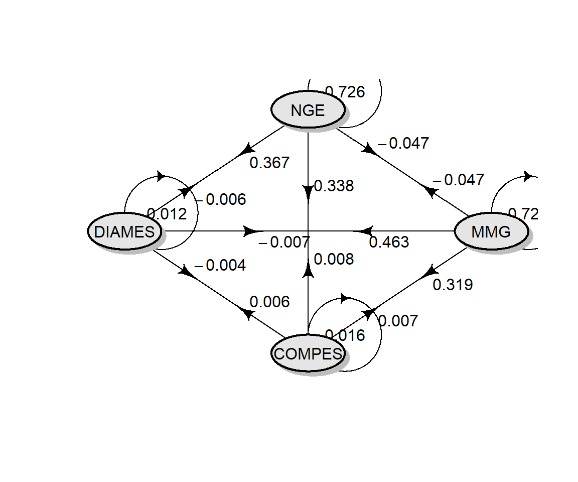
# diagrama de trilha
library(diagram)
## Carregando pacotes exigidos: shape
pcoeff5 <-
path_coeff(df_ge,
resp = MGE,
pred = c(MMG, COMPES, DIAMES, NGE))
## Weak multicollinearity.
## Condition Number = 24.907
## You will probably have path coefficients close to being unbiased.
coeffs <-
pcoeff5$Coefficients %>%
remove_cols(linear) %>%
round_cols(digits = 3)
coeffs
## MMG COMPES DIAMES NGE
## MMG 0.721 0.007 -0.007 -0.047
## COMPES 0.319 0.016 -0.004 0.338
## DIAMES 0.463 0.006 -0.012 0.367
## NGE -0.047 0.008 -0.006 0.726
plotmat(coeffs,
curve = 0,
box.size = 0.08,
box.prop = 0.5,
box.col = "gray90",
arr.type = "curved",
arr.pos = 0.35,
arr.lwd = 1,
arr.length = 0.4,
arr.width = 0.2)
Correlações canônicas
Em primeiro lugar, renomearemos as características relacionadas à planta ALT_PLANT e ALT_ESP com o sufixo _PLANTA para mostrar a usabilidade do select helper contains().
data_cc <-
  df_ge %>%
  rename(ESP_COMPES = COMPES,
         ESP_DIAMES = DIAMES,
         ESP_COMPSAB = COMP_SAB,
         GRAO_MGE = MGE,
         GRAO_MMG = MMG)

# Digitar os nomes das variáveis
cc1 <- can_corr(data_cc,
                FG = c(GRAO_MGE, GRAO_MMG),
                SG = c(ESP_COMPES, ESP_DIAMES, ESP_COMPSAB))
## ---------------------------------------------------------------------------
## Matrix (correlation/covariance) between variables of first group (FG)
## ---------------------------------------------------------------------------
##           GRAO_MGE  GRAO_MMG
## GRAO_MGE 1.0000000 0.6730371
## GRAO_MMG 0.6730371 1.0000000
## ---------------------------------------------------------------------------
## Collinearity within first group
## ---------------------------------------------------------------------------
## Weak multicollinearity in the matrix
## CN = 5.117
## Matrix determinant: 0.547021
## Largest correlation: GRAO_MGE x GRAO_MMG = 0.673
## Smallest correlation: GRAO_MGE x GRAO_MMG = 0.673
## Number of VIFs > 10: 0
## Number of correlations with r >= |0.8|: 0
## Variables with largest weight in the last eigenvalues:
## GRAO_MGE > GRAO_MMG
## ---------------------------------------------------------------------------
## Matrix (correlation/covariance) between variables of second group (SG)
## ---------------------------------------------------------------------------
##             ESP_COMPES ESP_DIAMES ESP_COMPSAB
## ESP_COMPES   1.0000000  0.3851451   0.2554068
## ESP_DIAMES   0.3851451  1.0000000   0.6974629
## ESP_COMPSAB  0.2554068  0.6974629   1.0000000
## ---------------------------------------------------------------------------
## Collinearity within second group
## ---------------------------------------------------------------------------
## Weak multicollinearity in the matrix
## CN = 6.679
## Matrix determinant: 0.4371931
## Largest correlation: ESP_DIAMES x ESP_COMPSAB = 0.697
## Smallest correlation: ESP_COMPES x ESP_COMPSAB = 0.255
## Number of VIFs > 10: 0
## Number of correlations with r >= |0.8|: 0
## Variables with largest weight in the last eigenvalues:
## ESP_DIAMES > ESP_COMPSAB > ESP_COMPES
## ---------------------------------------------------------------------------
## Matrix (correlation/covariance) between FG and SG
## ---------------------------------------------------------------------------
##          ESP_COMPES ESP_DIAMES ESP_COMPSAB
## GRAO_MGE  0.6685601  0.8241426   0.4709310
## GRAO_MMG  0.4421011  0.6419870   0.6187001
## ---------------------------------------------------------------------------
## Correlation of the canonical pairs and hypothesis testing
## ---------------------------------------------------------------------------
##            Var  Percent       Sum      Corr  Lambda     Chisq DF p_val
## U1V1 0.8430909 79.09135  79.09135 0.9181998 0.12194 319.84591  6     0
## U2V2 0.2228801 20.90865 100.00000 0.4721018 0.77712  38.32842  2     0
## ---------------------------------------------------------------------------
## Canonical coefficients of the first group
## ---------------------------------------------------------------------------
##                   U1         U2
## GRAO_MGE -0.98237574  0.9289894
## GRAO_MMG -0.02591325 -1.3518180
## ---------------------------------------------------------------------------
## Canonical coefficients of the second group
## ---------------------------------------------------------------------------
##                     V1         V2
## ESP_COMPES  -0.4445443  0.1353212
## ESP_DIAMES  -0.8650570  0.6712820
## ESP_COMPSAB  0.1955781 -1.3476588
## ---------------------------------------------------------------------------
## Canonical loads of the first group
## ---------------------------------------------------------------------------
##                  U1          U2
## GRAO_MGE -0.9998163  0.01916566
## GRAO_MMG -0.6870886 -0.72657362
## ---------------------------------------------------------------------------
## Canonical loads of the second group
## ---------------------------------------------------------------------------
##                     V1          V2
## ESP_COMPES  -0.7277648  0.04966103
## ESP_DIAMES  -0.8998626 -0.21654173
## ESP_COMPSAB -0.5213067 -0.84490257

# usando select helpers
cc2 <- can_corr(data_cc,
                FG = contains("GRAO_"),
                SG = contains("ESP_"))
## ---------------------------------------------------------------------------
## Matrix (correlation/covariance) between variables of first group (FG)
## ---------------------------------------------------------------------------
##           GRAO_MGE  GRAO_MMG
## GRAO_MGE 1.0000000 0.6730371
## GRAO_MMG 0.6730371 1.0000000
## ---------------------------------------------------------------------------
## Collinearity within first group
## ---------------------------------------------------------------------------
## Weak multicollinearity in the matrix
## CN = 5.117
## Matrix determinant: 0.547021
## Largest correlation: GRAO_MGE x GRAO_MMG = 0.673
## Smallest correlation: GRAO_MGE x GRAO_MMG = 0.673
## Number of VIFs > 10: 0
## Number of correlations with r >= |0.8|: 0
## Variables with largest weight in the last eigenvalues:
## GRAO_MGE > GRAO_MMG
## ---------------------------------------------------------------------------
## Matrix (correlation/covariance) between variables of second group (SG)
## ---------------------------------------------------------------------------
##             ESP_COMPES ESP_DIAMES ESP_COMPSAB
## ESP_COMPES   1.0000000  0.3851451   0.2554068
## ESP_DIAMES   0.3851451  1.0000000   0.6974629
## ESP_COMPSAB  0.2554068  0.6974629   1.0000000
## ---------------------------------------------------------------------------
## Collinearity within second group
## ---------------------------------------------------------------------------
## Weak multicollinearity in the matrix
## CN = 6.679
## Matrix determinant: 0.4371931
## Largest correlation: ESP_DIAMES x ESP_COMPSAB = 0.697
## Smallest correlation: ESP_COMPES x ESP_COMPSAB = 0.255
## Number of VIFs > 10: 0
## Number of correlations with r >= |0.8|: 0
## Variables with largest weight in the last eigenvalues:
## ESP_DIAMES > ESP_COMPSAB > ESP_COMPES
## ---------------------------------------------------------------------------
## Matrix (correlation/covariance) between FG and SG
## ---------------------------------------------------------------------------
##          ESP_COMPES ESP_DIAMES ESP_COMPSAB
## GRAO_MGE  0.6685601  0.8241426   0.4709310
## GRAO_MMG  0.4421011  0.6419870   0.6187001
## ---------------------------------------------------------------------------
## Correlation of the canonical pairs and hypothesis testing
## ---------------------------------------------------------------------------
##            Var  Percent       Sum      Corr  Lambda     Chisq DF p_val
## U1V1 0.8430909 79.09135  79.09135 0.9181998 0.12194 319.84591  6     0
## U2V2 0.2228801 20.90865 100.00000 0.4721018 0.77712  38.32842  2     0
## ---------------------------------------------------------------------------
## Canonical coefficients of the first group
## ---------------------------------------------------------------------------
##                   U1         U2
## GRAO_MGE -0.98237574  0.9289894
## GRAO_MMG -0.02591325 -1.3518180
## ---------------------------------------------------------------------------
## Canonical coefficients of the second group
## ---------------------------------------------------------------------------
##                     V1         V2
## ESP_COMPES  -0.4445443  0.1353212
## ESP_DIAMES  -0.8650570  0.6712820
## ESP_COMPSAB  0.1955781 -1.3476588
## ---------------------------------------------------------------------------
## Canonical loads of the first group
## ---------------------------------------------------------------------------
##                  U1          U2
## GRAO_MGE -0.9998163  0.01916566
## GRAO_MMG -0.6870886 -0.72657362
## ---------------------------------------------------------------------------
## Canonical loads of the second group
## ---------------------------------------------------------------------------
##                     V1          V2
## ESP_COMPES  -0.7277648  0.04966103
## ESP_DIAMES  -0.8998626 -0.21654173
## ESP_COMPSAB -0.5213067 -0.84490257
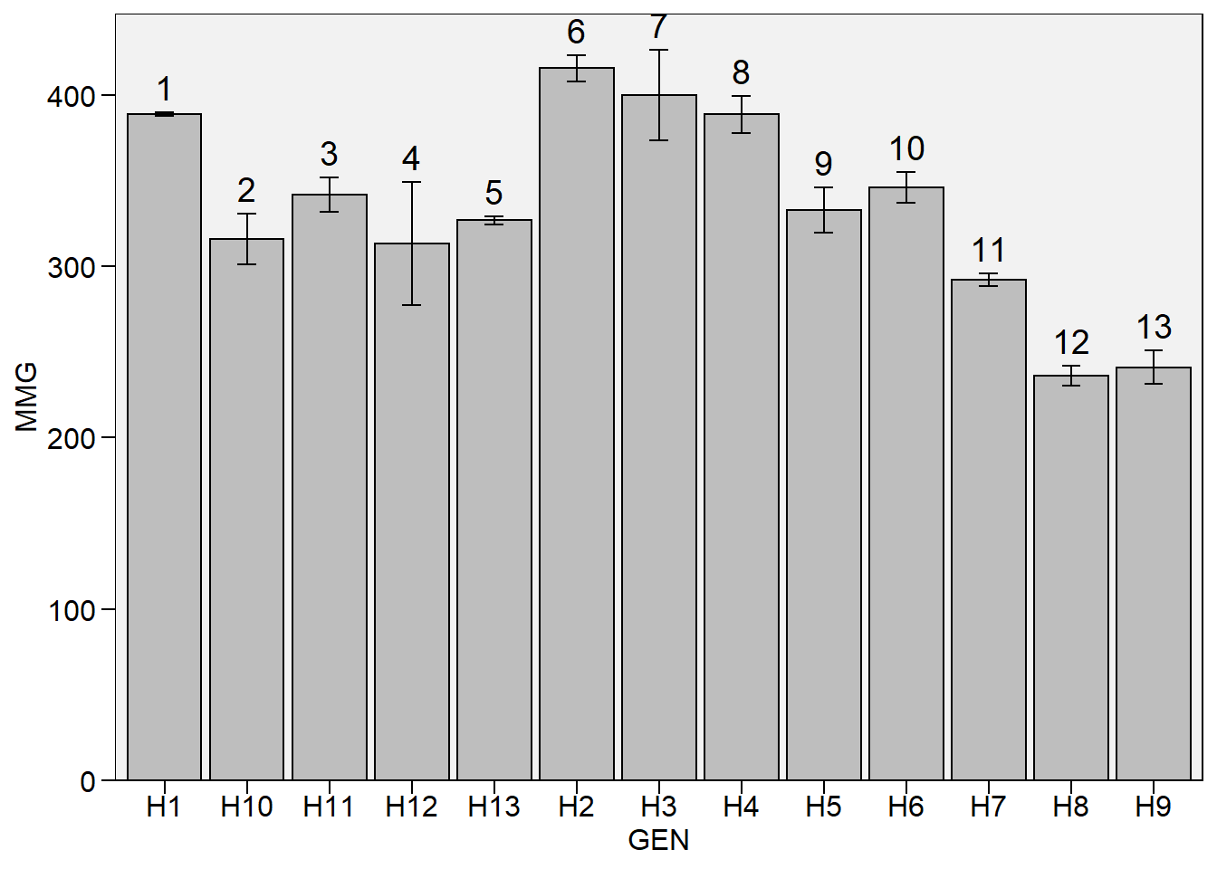
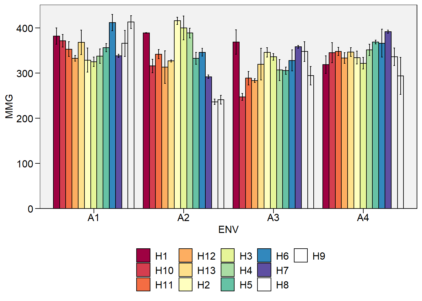
Gráfico de barras
plot_bars(df_g,
          x = GEN,
          y = MMG,
          lab.bar = 1:13)
plot_factbars(df_ge, ENV, GEN, resp = MMG)
## Warning in RColorBrewer::brewer.pal(n, pal): n too large, allowed maximum for palette Spectral is 11
## Returning the palette you asked for with that many colors
-
Olivoto, T., Souza, V. Q., Nardino, M., Carvalho, I. R., Ferrari, M., Pelegrin, A. J., Szareski, V. J., & Schmidt, D. (2017). Multicollinearity in path analysis: A simple method to reduce its effects. Agronomy Journal, 109(1), 131–142. https://doi.org/10.2134/agronj2016.04.0196 ↩︎